Ask the Heat Treat Doctor®: What Is Stress Relief and Why Perform It?

May 13, 2025 / STRESS RELIEVING TECHNICAL CONTENT

The Heat Treat Doctor® has returned to offer expert advice to Heat Treat Today readers and to answer your questions about heat treating, brazing, sintering, and other types of thermal treatments as well as questions on metallurgy, equipment, and process-related issues.

This informative piece was first released in Heat Treat Today’s May 2025 Sustainable Heat Treat Technologies print edition.

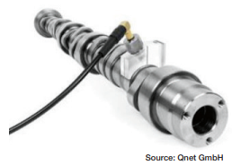
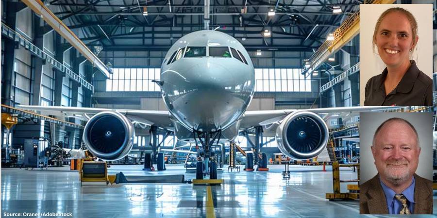
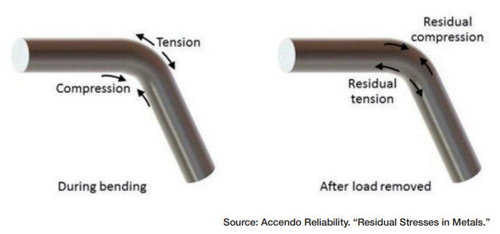
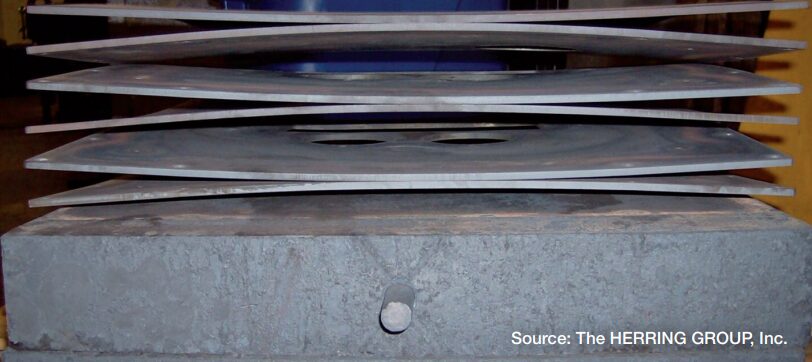
Stress relief is a heat treatment operation primarily intended to reduce or redistribute the internal stresses present in steel and other materials that were introduced from various manufacturing processes like bending (see Figure 1), drawing, rolling, shearing, forging, sawing, machining, grinding, milling, tuning, welding, etc., as well as from prior mill processing. The application end use of a part ultimately defines its allowable stress state. So, what is it, and how does one perform a stress relief operation? Let’s learn more.

Figure 1. Type of plastic deformation and residual stress during bending

How Does It Work?

Processes that depend on slow cooling (e.g., annealing, normalizing, stress relief) do so for a variety of reasons: to soften a material for subsequent operations (e.g., machining), to improve chemical homogeneity, to refine grain size, to relieve stresses, and for such reasons as embrittlement relief or magnetic properties (see Haga, L. J.). Residual stresses can compromise a material’s mechanical properties, leading to issues such as warping, cracking, and premature failure under service loads. As a general rule, the larger or more complex the part and/or the more aggressive certain manufacturing processes, the greater the amount of internal stress present.

Stress relief can be differentiated from other slow cooling processes in that it is most o en performed below the lower critical temperature (Ac1). Time at temperature depends on such factors as the complexity of the part, and enough time must be allowed to achieve the desired reduction in residual stress level. Following stress relief, the steel is cooled at a sufficiently slow rate to avoid formation or reintroduction of excessive thermal stresses. The stress relief process should be designed to reduce or eliminate internal stresses in a material without significantly altering its microstructure.

Stress relief helps improve a material’s stability, especially in applications where parts are subjected to cyclic or dynamic loading, since residual stresses can lead to fatigue failure over time. Stress relief helps to reduce these stresses, thus improving the material’s fatigue resistance and overall stability. During processes like welding, casting, or machining, the rapid cooling of steel can result in uneven contraction, leading to distortion in the final part. Stress relief helps reduce distortion, ensuring the part maintains its intended dimensions and shape.

Stress relief is particularly important after welding, which can introduce a significant amount of residual stress again resulting in distortion and/or cracking in service if not negated. Stress relief helps to minimize these effects and ensures the structural integrity of welded components.

How Do We Perform a Stress Relief Operation?

For carbon and alloy steels, stress relief operations are typically performed at 105°F–165°F (40°C–75°C) below the lower critical temperature, that is in the range of 930°F–1200°F (500°C–650°C). It is also important to understand the elimination of stress is not instantaneous, being a function of both temperature and time for maximum benefit. Typically, soak times of one hour per inch (25 mm) of maximum cross-sectional area (once the part has reached temperature) are recommended, with most soak times being in the range of 30 minutes to 2 hours, depending on the size and thickness of the part. Larger parts or components with complex geometries may require longer holding times to ensure uniform stress relief throughout the entire part. Alloy steels, especially if used in highstress environments (e.g., turbines, pressure vessels) benefit significantly from stress relief to improve their durability and fatigue resistance.

After removal from the furnace or oven, the parts rely on slow cooling to achieve a minimal residual stress state — the desired effect. Parts are typically still air cooled. Rapid cooling will only serve to reintroduce stress and is the most common mistake made in stress relief operations. A properly performed stress relief cycle often removes more than 90% of the internal stresses.

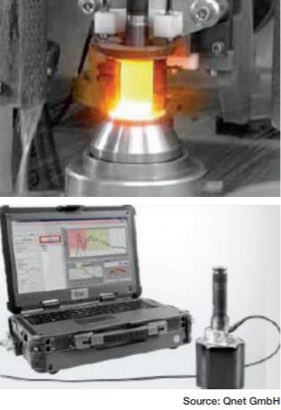
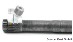
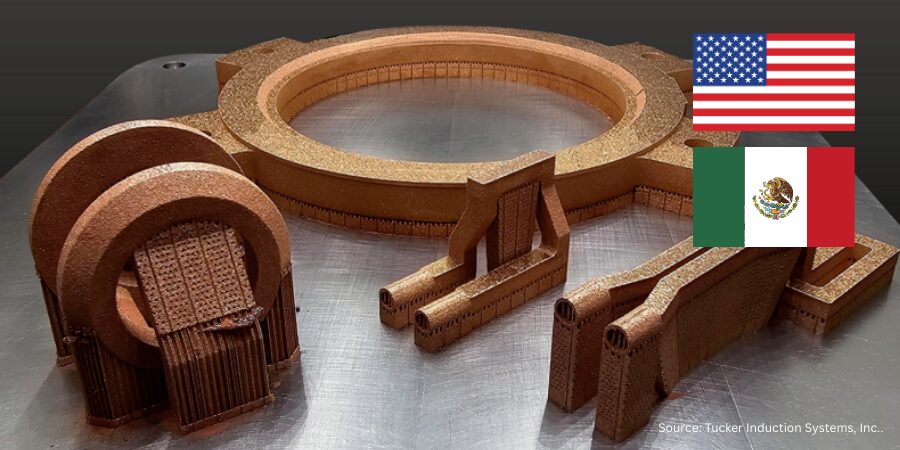
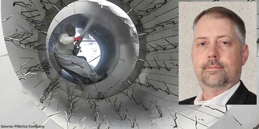
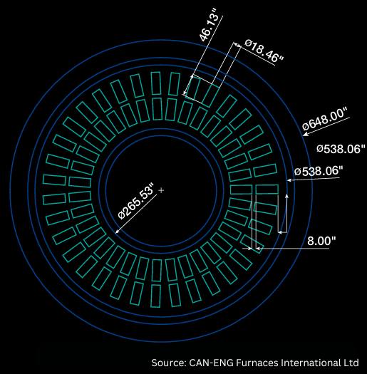
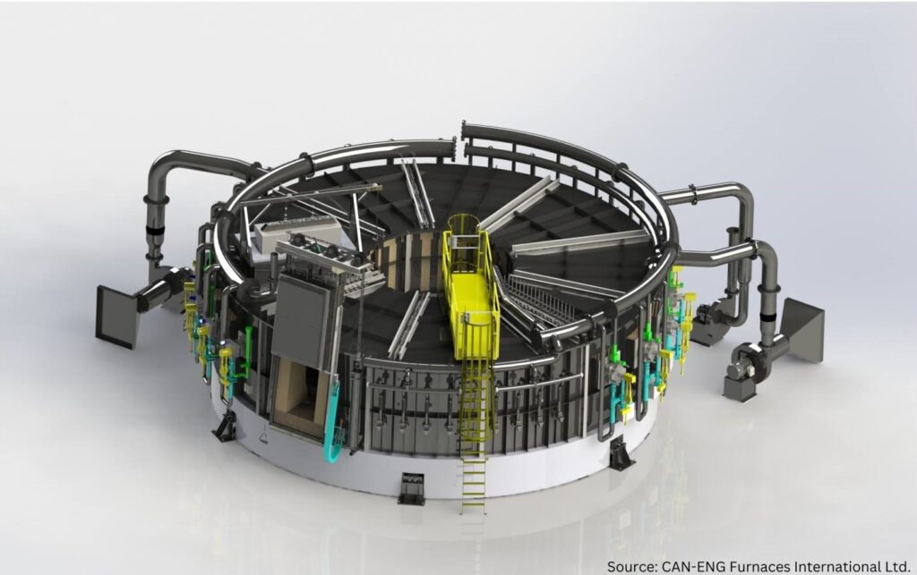
For tool steels the process is similar; it is common to perform a stress relief operation in the temperature ranges of 925°F–1025°F (500°C–550°C) for most tool steels or 1115°F–1300°F (600°C–700°C) for hot work and high-speed grades, allowing the parts to slowly cool to room temperature before subsequent operations. For stainless steels, the situation is more complex (see Atmosphere Heat Treatment, Volume 1 and ASM International’s Metals Handbook). Stress relief is done in the range of 550°F–800°F (290°C–425°C), which is below the sensitization range to avoid precipitation of carbides and reduced corrosion resistance. The operation depends on the form of the material, the operation being performed (e.g., machining), or if a completed assembly is to have a stress relief performed on it (Figure 2).

Figure 2. A combination of factors contributed to excessive warpage of 300 series stainless steel plates (including the method of fixturing used, the stress relief temperature selected, and the manufacturing process used to cut the plates).

At stress relief temperature, atomic movement increases, allowing the material to “rearrange” its internal structure, thus effectively relieving internal stresses. Steel is usually held at the stress relief temperature to ensure the remaining stresses are evenly distributed and reduced.

How Slow Is Slow?

Once the desired stress relief temperature has been reached and the part held for the appropriate time, the steel is then cooled slowly, typically in air, to prevent reintroduction of new thermal stresses. Rapid cooling (such as quenching) is to be avoided. A “still air cool” is often recommended, being defined as cooling at a rate of 40°F (22°C) per minute or faster to 1100°F (593°C) and then at a rate of 15°F–25°F (8°C–14°C) per minute from 1100°F–300°F (593°C–150°C). Below 300°F (150°C), any cooling rate may be used.

Poor Man’s Stress Relief

In hardening, rapid cooling/quenching alone or in combination with pre-existing internal stresses can result in unwanted distortion and even brittle fracture near welds in certain grades of metal. Stress corrosion cracking is another concern. For these reasons, a number of heat treaters introduce a “stress relief hold” during hardening or case hardening treatments. This involves heating of a workload to an intermediate temperature, in the range of 1000°F–1300°F (538°C–705°C) and soaking for a period of time equivalent to one hour per inch of maximum cross-sectional area. The idea is to allow for stress relaxation so that more predictable dimensional change occurs on quenching.

Types of Stress Relief Operations

While the basic process parameters for stress relief are largely the same, various types of methods can be used to achieve the desired results. Depending on the size and type of components being treated, one can use:

Batch furnaces where the load sits in the furnace or oven while being heated and soaked. This often allows precise control of these process variables. The load is then removed from the furnace for cooling.
Continuous furnaces where large volumes of component parts are moved through a heated section (usually but not always with multiple control zones) and then conveyed into one or more cooling sections as parts move through the furnace. The cooling sections are typically 2–2½ times the length of the heated section for adequate cooling time.
Induction heating for localized stress relief or when dealing with large or irregularly shaped components where heating the entire component part may not be desired. Stresses can be relieved in precise locations without affecting the entire part.
Vibratory Stress Relief, which uses mechanical vibration to redistribute residual stresses without the need for high temperature treatments. This technique has been used on castings and in some cases large, welded structures. The amount of stress relieved is often significantly less than thermal methods.
Post-Weld Heat Treatment (PWHT), often used during or after fabrication of welded steel structures. (Note: PWHT will be the subject of next month’s Ask The Heat Treat Doctor® column.)

In Summary

Stress relief is an oft-ignored but important heat treat process. By reducing internal stresses during manufacturing, stress relief operations help minimize post-heat treat distortion and improve mechanical properties. Understanding the significance of stress relief, selecting the best time/temperature cycles for a given material, and carefully controlling the process (especially as it relates to cooling rate) are keys to achieving the final result.

References

Accendo Reliability. “Residual Stresses in Metals.” Effective April 3, 2024. https://accendoreliability.com/residual-stresses-inmetals/. ASM International. “Metals Handbook, 10th ed., vol. 4, Heat Treating, Cleaning and Finishing.” (1991).

Grenier, Mario and Roger Gingras. “Rapid Tempering and Stress Relief Via High-Speed Convection Heating.” Industrial Heating, May 2003.

Haga, L. J., “Understanding Slow Cooling: Part 1 — Stress Relief.” Heat Treating, (October 1980).

Hebel, Thomas E. “Sub-harmonic Stress Relief Improves Mold Quality.” Mold Making Technology, 2009.

Herring, Daniel H. Atmosphere Heat Treatment, vol. I. BNP Media, 2014.

Herring, Daniel H. “Stress Relief.” Wire Forming Technology International (Summer 2010).

Lindqvist, Stefan and Jonas Holmgren. “Alternative Methods for Heat Stress Relief.” Master’s Thesis, Lulea University of Technology, 2007.

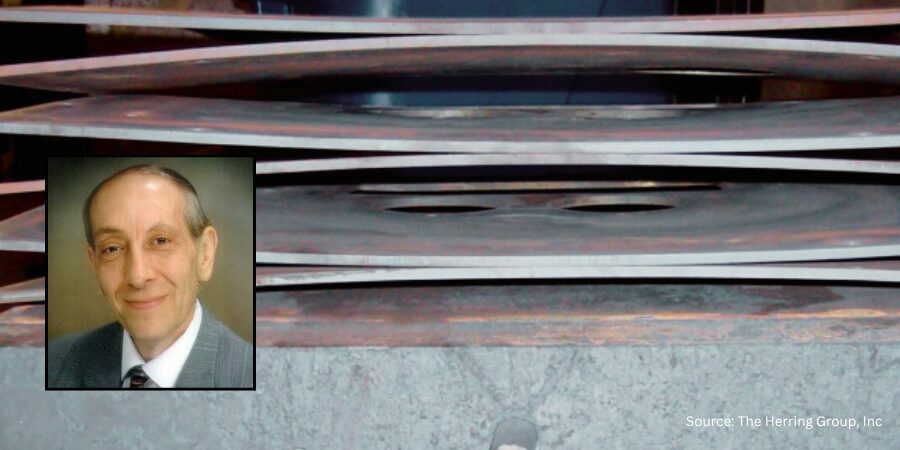
About the Author

Dan Herring
“The Heat Treat Doctor”
The HERRING GROUP, Inc.

Dan Herring has been in the industry for over 50 years and has gained vast experience in fields that include materials science, engineering, metallurgy, new product research, and many other areas. He is the author of six books and over 700 technical articles.

For more information: Contact Dan at dherring@heat-treat-doctor.com.

For more information about Dan’s books: see his page at the Heat Treat Store.

Find Heat Treating Products And Services When You Search On Heat Treat Buyers Guide.Com

Ask the Heat Treat Doctor®: What Is Stress Relief and Why Perform It? Read More »

Induction Hardened Case Depth Measurement Using Ultrasonic Backscattering

May 6, 2025 / INDUCTION HEATING TECHNICAL CONTENT

By Jose Miguel Equihua Toral, Head of the New Projects and Development, BOINSA Mexico and Manager, InTech NDT, USA.

Nondestructive testing (NDT) techniques have been used exclusively to detect defects in structures and components after they have been manufactured. To protect public safety and security, it is imperative to test parts efficiently and ensure their quality. Nondestructive evaluation, like ultrasonic backscattering, serves an important role in this area.

This informative piece was first released in Heat Treat Today’s April 2025 Annual Induction Heating & Melting print edition.

Introduction

Figure 1a. Induction hardening (top)
Figure 1b. UT backscattering testing (bottom)

Induction hardening is a critical process in manufacturing automotive, agricultural, and aeronautical components, such as crankshafts, camshafts, constant velocity joints, and axle shafts (Figure 1a). The procedure for the evaluation of metallurgical characteristics is carried out in the laboratory and is destructive testing (Bernard, “Methods of Measuring Case Depth in Steels”). This means the component will be unusable. Additionally, this procedure is time-consuming, expensive, and cannot be integrated into the production line. Over time, the industry has sought faster and more efficient methods to evaluate metallurgical characteristics, such as eddy current testing, magnetic methods, and ultrasound. Having the capability of monitoring material properties after each key process can help minimize the cost of processing out-of-specification material. A combination of nondestructive testing methods can help to guarantee the quality of induction heat treatment operations (ASM Handbook, vol 4c).

Ultrasonic methods, for example, can be used to determine microstructural differences in metals. For this, contact testing with pulse-echo technique is used. For inductive-hardened parts, the ultrasonic backscattering method works because the hardened layer (martensite) is almost transparent to ultrasonic waves (in range of 20 MHz), while bulk material (ferrite-pearlite) scatters ultrasonic waves very strongly.

In this article, we will address the use of industrial ultrasound applying the backscattering technique, which offers a direct determination of the depth. This method is simple and does not require prior calibration to evaluate the components (Figure 1b).

The Ultrasonic Backscattering Technique

Figure 2a. Ultrasonic backscattering technique (top)
Figure 2b. Time-of-flight measurement (bottom)

Iron crystals exhibit notable acoustic anisotropy, meaning the acoustic velocity (c) varies depending on the direction of travel within the crystal. Grain boundaries represent transitions between crystal structures with varying orientations. The resulting variation in impedance causes the ultrasonic pulse to scatter at the grain boundaries. The ultrasonic technique for measuring hardness depths (SHD) utilizes this grain boundary scattering effect. This technique is known as the ultrasonic backscattering method (Kruger et al., “Broadband Ultrasonic Backscattering”).

The ultrasonic backscattering method for hardness depth testing relies on finding the ultrasound frequency that does not scatter at the fine-grained hardened microstructure of the outer layer but at the coarse-grained core material (Figure 2a). The different scattering properties from the varied grain sizes of the hardened surface layer and the core material are seen in the backscattering measurement. The connection between scattering and the material’s grain size is utilized to produce a detectable backscattering echo when the ultrasound penetrates the core material.

The depth (SHD_US) of the interface can be determined using the time (t) it takes for the sound pulse to reach the scattering interface, the angle of the shear wave (βT), and the velocity (c) of the shear wave in steel. Therefore, the following equation is relevant for a flat shape:

SHD_US=1/2∙c∙t∙cos∙βT

Based on this equation, the acoustically measured surface hardness depth (SHD_US) is always found before the sound exit point of the probe wedge. To guarantee an accurate measurement of this location during destructive testing, this distance (A) must be calculated. The next equation is used for a plane geometry:

A=1/2∙c∙t∙sin∙βT

The backscattered ultrasonic amplitude depends on the actual gradient of the microstructure. In the transition zone, grain boundaries, grain size, and second phases change the acoustic impedance value discontinuously, depending on the ultrasonic frequency. Different backscattering signals in the hardened and bulk material occur (Yanming Guo, “Effects of material”). Th ese amplitude characteristics can be used to evaluate the case depth by using simple time-of-flight measurements (Figure 2b). Contact testing is generally done by using portable equipment, using a contact wedge where the transducer is mounted to be inclined at a certain angle, and shear waves are emitted into the component. Ultrasonic backscatter takes place at the surface of the component due to surface roughness and results in the return of the energy to the transducer (first echo). Ultrasonic energy enters the hardened surface layer made of fine martensitic structure, and thus, no scatter of ultrasonic waves takes place in this region. However, when the shear waves reach the transition zone where martensitic structure is gradually converted into ferrite-pearlite structure, which has a larger grain size, once again energy is scattered at the grain boundaries, and the transition zone backscatter forms the second echo. The difference in time-of-flight of these two echoes is proportional to the case depth of the component.

Technical Requirements

Technical requirements for testing hardness depth using the ultrasonic backscattering method will produce optimal results in the following conditions:

The test parts should be induction-hardened.
The test parts must be forged, not cast.
There is minimal or no microstructure present between the hardened martensitic microstructure and the core material.
The grain size of the core material is significantly larger than the grain size of the hardened microstructure, leading to considerable backscattering of shear waves at a frequency of 20 MHz.
The minimum hardness depth that can be measured is 1.2 mm. Smaller hardness depths need special considerations, such as adjustments to the wedge design.

Practical Correlation Between NDT and DT

Destructive hardness depth testing is a method to determine the thickness of the case depth of hardened parts. In the process, the parts are destroyed, or their surface is altered rendering each tested part unusable. Hardness depth profiles are usually determined by using the Vickers test to measure the hardness of a reference sample at different points in a line from the surface to the core.

If you compare the acoustically measured surface hardness depth SHD_US with the surface hardness depth measured with destructive methods SHD_DT, you will see a basic difference: Independent of the hardness limit and the minimum hardness, the acoustic testing always determines the depth of the core material that has not been affected by the hardening process. As a consequence, this value tends to be slightly higher than the surface hardness depth measured with destructive methods SHD_DT. This difference can be compensated by means of a correction term ΔT (“Off set”):

SHD_US = SHD_DT – ΔT

In the case of hardness curves with rapidly decreasing hardness values just above the interface, the transit time is measured at 20% of the height of the backscattering signal’s amplitude, and the results of the acoustic and the destructive hardness depth tests will match. The reason for this is the slightly shorter sound path in the marginal ray of the divergent sound field, which induces the backscattering echo.

If cases occur regularly in which the hardness curve deviates significantly from the characteristics, reference tests must be conducted to determine the correction factor ΔT. Reasons for this could be material and/or process related. The calculated correction factor can then be integrated in the respective test task as a test parameter.

Technical Description and Measurement Highlights

The manual device includes a four-channel ultrasonic board managed by a software package for program settings, signal processing, reporting, and overall quality assurance requirements. The parts are put together in an industrial notebook meant for tough industrial settings. The probe systems allow testing of components with complex shapes. The wedge of the probe system is adjusted to fit the geometry of the specific test location. Testing can be done before or after machining.

The primary cause of measurement error is the evaluation of surface position; the shape of the surface signal relies on proper coupling and the operator’s skill. Another source of error is the placement of the marker that indicates the time-of-flight when the pulse hits the interface. The sharper the signal rises, the less the error. Therefore, a shear wave angle as low as reasonable is employed, and scanning in the direction of decreasing SHD is advised. Achievable accuracy of better than ±0.1 mm is possible for standard parts with high-quality surfaces. Nevertheless, the operator must monitor the “good” shape of the A-scan during data collection. Accuracy based on microindentation hardness profiles compared to the backscatter method is slightly lower, estimated at ±0.2 mm on average, based on the material microstructure (Bogaerts et al., “Surface Hardness Depth Measurement”). We are able to test different geometries like crankshafts (Figure 3), camshaft s (Figure 4), tulips (Figure 5), and barshafts (Figure 6), to mention some components.

Feasibility Testing

Situation: During induction hardening, an unanticipated variation on the case depth was detected on the shaft of an axle bar (Figure 7). We were requested to examine the case depth in this important area using a P3123 Hardness Depth Tester to find out if the case depth met specifications.

Figure 7. Induction case-depth variation

Results: During the testing, we noted the case depth was insufficient compared to the minimum required case depth of 5.5 mm. This meant all induction hardened parts made before the discovery had to be paused while a complete check of the case depth was performed. All axle bars hardened after the discovery were analyzed (Figure 8), starting with the most recently hardened parts. Case depth was also evaluated by making a microindentation hardness profile in the hardened area, showing a case depth consistent between ultrasound readings with the P3123 and the destructive testing measurements. In Figure 9, we can observe the measurement of the out of specification case depth, and in Figure 10, we have the measurement within specification case depth.

Hardness depth testers are used for optimizing production parameters, reducing downtimes after inductor changes, fast production control, and quality management. The techniques discussed in this article offer the technical advantages to ensure quality assurance for both steel and induction hardened components. Feasibility testing is required, which can be performed with prompt review of the ultrasound behavior in components.

Figure 10. Case depth within specification

Figure 9. Case depth out of specification

References

ASM International. ASM Handbook Volume 4C: Induction Heating and Heat Treatment. 2014.

Bernard, William J. “Methods of Measuring Case Depth in Steels.” Steel Heat Treating Fundamentals and Processes (2013): 405-416. https://doi.org/10.31399/asm.hb.v04a.a0005795.

Bogaerts, Mike, Michael Kroening, Paul Kroening, and Tobias Mueller. “Surface Hardness Depth Measurement Using Ultrasound Backscattering.” AM&P Technical Articles 177, no. 8 (2019): 58-62. https://doi.org/10.31399/asm.amp.2019-08.p058.

Guo, Yanming. “Eff ects of material microstructure and surface geometry on ultrasonic scattering and fl aw detection.” Dissertation, Iowa State University, 2003.

Kruger, S.E., J.M.A. Rebello, and J. Charlier. “Broadband Ultrasonic Backscattering Applied to Nondestructive Characterization of Materials.” IEEE Transactions on Ultrasonics, Ferroelectrics and Frequency Control 51, no. 7 (2004): 832-838. https://doi.org/10.1109/tu c.2004.1320742.

About The Author:

Jose Miguel Equihua Toral
Head of New Projects and Development
BOINSA Mexico
Manager,
InTech NDT, USA

Jose Miguel Equihua Toral graduated as a mining engineer from Guanajuato University and obtained his Master’s Degree in Engineering from the National Technology Institute of Mexico. He currently works as head of the new projects and development department of BOINSA de Mexico, involved in technological and operational advances in the design, manufacture, and repair of induction coils, as well as advances in the application of non-destructive testing methods for the quality assurance of components for the automotive, agricultural, and energy industries. This experience has led to the formation of InTech NDT, to serve the U.S. market.

For more information: Contact Jose Miguel Equihua Toral at miguel.equihua@intech-ndt.com.

Find heat treating products and services when you search on Heat Treat Buyers Guide.Com

Induction Hardened Case Depth Measurement Using Ultrasonic Backscattering Read More »

Applied Machine Learning and Optimization in Steel Melting

April 29, 2025 / FOUNDRY CASTING TECHNICAL CONTENT

What data can be gleaned for optimizing charge combinations? Check out this Technical Tuesday installment, by Tim Kaufmann and Dierk Hartmann, of Hochschule für angewandte Wissenschaften Kempten; Shikun Chen and Johannes Gottschling, of Universität Duisburg-Essen.

This article showcases the utilization of data-driven modeling assisted by machine learning (ML) to simulate the melting process of different steel grades in a medium-frequency induction furnace concerning the target variable of energy consumption. The results of the predictive models developed are presented in this article, along with the possibility of producing optimized charge combinations through the use of predictive outcomes and backward analysis.

This informative piece was first released in Heat Treat Today’s April 2025 Annual Induction Heating & Melting print edition.

Introduction

The steel and foundry industry faces several ongoing challenges, such as escalating costs of raw materials and energy, CO₂ emission regulations, and fierce global competition. To tackle these challenges, there is a continual demand for improving current production processes. Despite the strides made by smelters and equipment manufacturers in enhancing plant technology, there is still room for improvement in production procedures and processes. One possible approach to enhancing these processes is through modeling.

In recent times, digitalization and machine learning (ML) have emerged as a promising modeling method, as demonstrated in material development or process optimization in the steel industry (Lee et al., “A Machine-Learning-Based Alloy,” 11012; Klanke et al., “Advanced Data-Driven Prediction,” 1307-1313; Yingjun et al., “A Machine Learning and Genetic,” 360-375.) The subsequent example showcases how the melting process in a medium-frequency induction furnace can be modeled with respect to energy consumption, using specific process data obtained from a steel foundry, and subsequently optimized through synthetic data generation and backward analysis.

Modeling

Various ML algorithms [including Random Forest, Extra Trees, LightGBM, XGBoost, MLP (Neural Network), K-Nearest Neighbors] were trained and their hyperparameters optimized for modeling Erikson et al., “Autogluon-tabular”. The hyperparameters are set before the learning process begins and influence how well a model can represent a process. Some examples of hyperparameters in ML are the learning rates, the number of hidden layers in a deep learning neural network, or the number of branches in a decision tree.

For the modeling, data from the process, induction furnace, and charge database of a medium-sized steel foundry were consolidated and pre-processed. The melting unit is a medium-frequency induction furnace with a capacity of approximately 7 tons. Figure 1 depicts an overview of the modeling workflow. The process and furnace databases contain data, such as the chemical analysis of the input raw materials, the measured melting time, and the measured melting energy requirement of the respective melts. The required melting energy (kWh), the required melting time (min) to reach the required tapping temperature, and the alloy quantities (Co, FeCr, FeV, FeSi, etc. kg) to be added after the melting process to correct the chemical analysis were selected as target values. The charge database contains data on the charge scrap for each melt, with details of its quantity and chemical analysis.

At the foundry, the scrap is roughly pre-sorted in separate bins so that the scrap used in a batch can be distinguished. As an intermediate step, the expected melting enthalpy of the scrap was calculated from the chemical analyses using simulation software (CALPHAD method). Based on the thermodynamic data, an ML model was trained to also consider the theoretically required melting enthalpy of the raw materials based on the chemical analysis. The measured raw data consist of approximately 10,000 individual melts of different steel grades. After pre-processing (removing outliers, formatting the data, etc.) and applying domain knowledge, about 70% of the data was used for process modeling. Domain knowledge in this context means reviewing and filtering the data with an understanding of the process. For example, some obvious outliers or erroneous data, such as negative charge quantities or charges of allegedly more than 7 tons of material, were not detected by the pre-processing algorithms and were manually filtered out.

Figure 1. Process modeling of the melting process *The ML Models are a function of the change of energy, melting time, and chemical composition of the ferro alloys

The remaining dataset contains information on approximately 7,000 individual steel melts with approximately 300 influencing variables (columns in the dataset influencing variables, also called “features”) of which approximately 200 are charge-relevant influencing variables. In addition, the steel scrap was divided into groups, such as recycled or foreign scrap and alloys, characterized based on its empirically assessed geometry (cut-offs, “bones,” plates, chipped scrap, etc.), and added to the dataset as information.

Table 1. Overview of the prediction metrics of the energy models for 1.2379 steel

The data were subsequently split as 70% training, 20% validation, and 10% test data. The algorithms were trained on the training data and then tested for prediction quality on the test data. This step is necessary because overfitting or underfitting can occur when training ML algorithms. This means that the models perform well on the training data but poorly on unknown future process data. The test data, representing completely unknown future process data or states, are separated beforehand. In each case between the prediction of the model and the “real” measured value of the respective melt in the test dataset, the prediction of the models was evaluated with the metrics MAE (mean absolute error), MSE (mean square error), RMSE (root mean square error), and R² (coefficient of determination).

The energy consumption during melting in an induction furnace depends on many factors, such as the raw materials being fed (fine or bulky material, impurities, etc.), the sequence in which they are charged, the actual process control (e.g., is the furnace lid open for an unnecessarily long time due to bulky scrap in the charge), and many other direct and indirect influencing factors. Due to this complexity, modeling

Figure 2. Result of the process model in terms of predicting the energy required to melt 1.2379 steel

Figure 3. Residuals of the energy model test data for 1.2379 steel

Figure 2 depicts the comparison of the values (1.2379 steel) of energy consumption (x-axis) predicted by the best ML model based on the input features and the actual measured values (y-axis) in the test and training datasets, respectively. For the training dataset the R² is 0.92 with an RMSE of 58 kWh, and for the test dataset, the R² is 0.69 with an RMSE of 119 kWh (Table 1). For the test data, this corresponds to a relative prediction error of about 5%–10%.

Figure 3 illustrates the residual distribution (difference between the actual measured value and the model prediction) of the 1.2379 energy model in the test dataset. The residual distribution gives an indication of the prediction quality of a model. If the expected value of the residuals is not close to zero and they are not approximately normally distributed, this means that the model has a systematic tendency to either over- or under-predict. Furthermore, if there is a pattern in the residuals, the model does not appear to be able to explain some relationships within the data and is therefore qualitatively inconsistent. In the generated model, the residuals are almost normally distributed, and the prediction error does not appear to follow any pattern, suggesting good prediction quality.

Charge Optimization

After a trained ML model has been prepared for use, backward analysis can be applied to the training dataset to determine the range of values of the independent variable that corresponds to a given target variable. Consequently, backward analysis offers an inverse function of the prediction function, which can be leveraged to determine optimized process values. In this scenario, the optimized process value is the charge composition, with the target variable being energy consumption.

There are multiple mathematical optimization methods that can be employed for this purpose based on a well-trained ML model. A straightforward and easy-to-understand approach is to create a dense set of independent process variables using linear interpolation within a given range, such as the minimum and maximum values of a variable. The target variable is subsequently predicted based on this set of generated variables. This method can be computationally intensive and time consuming, and it does not consider the hidden patterns within the dataset, resulting in some useful information being disregarded.

In order to capture the hidden information and accurately reflect the true value of the original data set, a deep learning-based method called SDV (Synthetic Data Vault) is used in this work Patki et al., “The Synthetic Data Vault,” 1-10. Various synthetic data generation algorithms, such as Gaussian copula, are used in the SDV library. Mathematically, a Gaussian copula is a distribution over the unit cube between 0 and 1 in dimensions generated by applying the probability integral transformation to a multivariate normal distribution over all real numbers (R). Intuitively, the Gaussian copula is a mathematical function that can describe the joint distribution of several random variables by analyzing the dependencies between their marginal distributions. It can learn the intrinsic information of the original dataset to generate new synthetic data that have the same format and statistical properties as the original dataset.

Figure 4. The KDE comparison of real and synthetic variable values of the target variable energy consumption

Since the SDV library learns probabilistic rules, most of the synthesized data is general. To improve the quality of the synthesized data, some technical constraints can be defined when generating the data. For example, constraints can be set so that the values of a column in the generated data set are always larger or smaller than another column. Figure 4 shows the comparison of the Kernel Density Estimation (KDE) of the target variable energy consumption in the real and synthetic data. The distributions are very similar. In the current production process, the SDV dataset can be used to quickly determine the values that best approximate the required quality according to the prediction for the independent variables. This selection can then be further optimized, for example, in terms of cost and energy efficiency.

Figure 5 illustrates the process of backward analysis and resulting optimization based on the target, the required chemical elements, and the amount of scrap that must be included in a melt to ensure the target composition. The aim of data-driven optimization is to determine the most cost-effective scrap mix or “recipe,” taking into account the predicted energy consumption and metal yield. The database, which contains information from scrap suppliers, is constantly updated and fed new data. Because of this, the results of the optimization are automatically adjusted on an ongoing basis.

Figure 5. Sequence of backward analysis and large-scale charge optimization

The solution to the programming problem should indicate from which scrap supplier and which type of scrap combinations should be purchased to maintain the desired stock levels of the steel producer that will meet the above conditions (desired chemical analysis, minimized energy consumption, post-gating with ferro-alloys) or minimize costs Goutam and Fourer, “A Survey of Mathematical Programming,” 387-400.

The availability of individual scrap suppliers, the market price, and the levels of elements, such as chromium, vanadium, sulfur, and phosphorus, all affect how economically recovered steel scrap can be used. To ensure that steel grades are consistent throughout the cast or semi-finished product and to meet a client’s criteria, such as weldability and hardness, it is critical to control the amount of these elements in the final melt.

A model-based linear first-order (LP) optimization problem has been developed as a tool for scrap purchasing decision makers Applegate et al., “Practical Large-Scale,” 20243-20257 and Miletic et al., “Model-Based Optimization,” 263-266. The computations are performed by the model using the results of the ML model shown earlier in terms of energy consumption and scrap quality data, market prices, and supplier availability information. Prices, quality, and supplier information are included in the model along with quality and density constraints and a production schedule. The LP considers the following convex quadratic programming problem:

where A is an m × n Matrix and Q is a symmetric and n × n positive semidefinite matrix. The vectors of the input features have the upper bounds u^c and u^v and the lower bounds l^c and l^v , which have values in R U+∞ and in R U–∞ respectively. This equation assumes that l^c ≤ u^c and l^v ≤ u^v. For example, it can take into account that a particular scrap is only used between 500 kg and 1,500 kg, which may be due to process-related circumstances, and is therefore added as a constraint to the optimization objective.

An approximate linear cost equation is used in the model. Scrap costs are determined by market prices and availability, as well as internal storage costs; energy costs are calculated by estimating the energy consumption predicted by the ML model for each type of scrap and the amount of electricity required. The work described above ends with a web-based user interface (Figure 6) that displays the concrete purchase plan. Transportation of the purchased scrap could be considered through route planning. Finally, an estimate of the quantitative carbon footprint of the melting process and the logistics of scrap delivery can be calculated and tracked.

Figure 6. Overview of the entire software: In the background, the software accesses the generated ML model and the database of available scrap and generates an optimized shopping list for the scrap. Factors such as energy consumption predicted by the ML model, scrap prices, calculated CO2 emissions, the distance, and desired chemical composition are considered.

Conclusion

This article has shown how the melting and purchasing process in the steel industry can be modeled and optimized using modern methods from the field of artificial intelligence and mathematical optimization methods. Based on the input features (the scrap composition and the process parameters), the generated models can predict the expected energy consumption with a relative error of about 5%–10%. The optimization software can then be used to generate a scrap composition. Here, the composition of the purchase list from a purely monetary point of view (scrap prices) is supplemented by the consideration of resource and energy efficiency.

The foundry and steel industry naturally must go through a large number of (partial) processes on the way from raw material to finished casting or semi-finished product, where a large amount of production data is generated. For a future data-driven optimization of foundry processes, it is therefore necessary to consolidate this data to make the available knowledge usable for process optimization with the help of tools such as ML. This can provide foundries and their staff with another useful tool, like casting simulation, to further improve existing processes and procedures.

References

Applegate, David, Mateo Díaz, Oliver Hinder, Haihao Lu, Miles Lubin, Brendan O’Donoghue, Warren Schudy. “Practical Large-Scale Linear Programming Using Primal-Dual Hybrid Gradient.” Advances in Neural Information Processing Systems 34 (2021): 20243-20257.

Dutta, Goutam, and Robert Fourer. “A Survey of Mathematical Programming Applications in Integrated Steel Plants.” Manufacturing & Service Operations Management 3, no. 4 (2001): 387-400.

Erickson, Nick, et al. “Autogluon-tabular: Robust and accurate automl for structured data.” arXiv preprint arXiv:2003.06505 (2020).

Klanke, Stefan, Mike Löpke, Norbert Uebber, and Hans-Jürgen Odentha. “Advanced Data-Driven Prediction Models for BOF Endpoint Detection.” Association for Iron & Steel Technology Proceedings (2017), 1307-1313.

Lee, Jin-Woong, Chaewon Park, Byung Do Lee, Joonseo Park, Nam Hoon Goo, and Kee-Sun Sohn. “A Machine-Learning-Based Alloy Design Platform Th at Enables Both Forward and Inverse Predictions for Thermo-Mechanically Controlled Processed (TMCP) Steel Alloys.” Scientific Reports 11, no. 1 (2021): 11012.

Miletic, I., R. Garbaty, S. Waterfall, M. Mathewson. “Model-Based Optimization of Scrap Steel Purchasing.” IFAC Proceedings 40, no. 11 (2007): 263-266.

Patki, Neha, Roy Wedge, and Kalyan Veeramachaneni. “Th e Synthetic Data Vault.” IEEE International Conference on Data Science and Advanced Analytics (DSAA) (2016): 1-10.

Yingjun Ji, Shixin Liu, Mengchu Zhou, Ziyan Zhao, Xiwang Guo, and Liang Qi. “A Machine Learning and Genetic Algorithm-Based Method for Predicting Width Deviation of Hot-Rolled Strip in Steel Production Systems.” Information Sciences 589 (2022): 360-375.

This article content is used with permission by Heat Treat Today’s media partner heat processing, which published this article in February 2023.

About The Authors:

For more information:
Contact Tim Kaufmann at tim.kaufmann@hs-kempten.de
Dierk Hartmann at dierk.hartmann@hs-kempten.de
Shikun Chen at shikun.chen@uni-due.de or
Johannes Gottschling at Johannes.gottschling@uni-due.de

Find heat treating products and services when you search on Heat Treat Buyers Guide.Com

Applied Machine Learning and Optimization in Steel Melting Read More »

Is There Too Much Air in Here

April 28, 2025 / BURNERS & COMBUSTION SYSTEMS TECHNICAL CONTENT, Manufacturing Heat Treat Technical Content, OP-ED

What’s the relationship between excess air and your bottom-line? In this article, Jim Roberts, President, U.S. Ignition, shares how to increase efficiency and reduce waste in your heat treating operations.

This informative piece was first released in Heat Treat Today’s April 2025 Annual Induction Heating & Melting print edition.

A furnace guy walks into a heat treat shop . . . and notices there is a little bit of a yelp to the burners, or the furnace operator mentions the furnace is slowing down on heat up recovery times from a cold load. Or, if you are responsible for fuel costs and monitoring the gas meters, you might notice that situation is slipping in the wrong direction. Or, the burners seem to be dumping soot on your floor. We discussed that in past columns — remember?

Well, it’s all got to do with air. It may seem odd to talk about air when the objective is to utilize fuel at an optimum efficiency, but that’s how we intend to get combustion under control. Let’s go after the air. You remember that we talked about making sure that combustion air sources (blowers, eductors, etc.) were all operating at optimum performance, so the air remains supplied as engineered when the equipment was new. So, now we have our air being delivered at the peak levels we want, but it looks like one of the air valves has shifted, which we covered in the last column on keeping the air sources clean.

This next little tidbit of information is intended to show us all how much this little-considered entity we call AIR can affect the bottom line. Here’s some info you might find interesting.

Eliminate Excess Air

If controls have moved or another phenomenon has caused the burners to lean out, it could cost you a fortune. Most burners are designed to burn with a small percentage of excess air (less than 15%).

Exceptions would include air heating equipment and low temperature drying operations where the excess air is used to control the temperature of the flame. If you operate a burner that has been designed to run at 10–15% excess air and the burner controls or settings drift into the range of 50% excess air (that is a difference of 2–3% O₂ or 7.5% O₂ in the products of combustion), the difference in an 1800°F oven operation is a calculated 9% loss of fuel efficiency. If you operate a 1 million BTU/hr burner, firing at 75% of the time six days a week for 50 weeks a year, your gas usage would be approx. 5400 therms a year. If we calculate that your gas costs (delivered) are in the range of $4 per 1,000 cu/ft, keeping one burner in tune would save approximately $1,950 per year.

What!!! If you are running a good-sized batch furnace with four burners, that’s a cool $7,800 dollars per year. A ten burner continuous line is going to save almost $20,000 dollars per year. All that just because you cared enough to check excess air levels regularly.

Of course, wasting fuel because you are heating air instead of product is a terrible thing. But don’t forget you can go the other way, too, and go fuel rich with the settings. Then, you take the chance of actually damaging equipment with the carbon you could be producing in a reducing (excess fuel) situation. Carbon can affect all sorts of equipment life, including shortening burner component life and reducing radiant tube and fixture life. It’s not good. Don’t do it. No excess air and no excess fuel will lead you to a happier and more profitable life.

As always, I recommend that you associate your business with the furnace and combustion technicians in your area who can help you make sure everything stays in tune. We’ll chat in the next edition of Heat Treat Today about how to keep a handle on this in-house, so you can tell your experts what you are seeing and start saving yourself gobs of fuel!

For more information: Contact Jim Roberts at jim@usignition.com

Find heat treating products and services when you search on Heat Treat Buyers Guide.Com

Is There Too Much Air in Here Read More »

How To Find Both Real and Virtual Vacuum Leaks

April 22, 2025 / Featured, HEAT TREATING EQUIPMENT, Manufacturing Heat Treat Technical Content, VACUUM FURNACES, VACUUM FURNACES TECHNICAL CONTENT

In this Technical Tuesday installment, Thomas Wingens, Founder & President, WINGENS CONSULTANTS; Dr. Dermot Monaghan, Managing Director, and Dr. Erik Cox, Manager of New Business Development, Gencoa, train readers for finding both real and evasive virtual vacuum leaks.

Leak detection is difficult enough with a “real” leak, but “virtual” leaks present their own challenges. To enhance cost savings and further process efficiencies, it’s essential to have leak sensor technology that can effectively monitor the vacuum chamber and pinpoint these problematic leaks.

This informative piece was first released in Heat Treat Today’s March 2025 Annual Aerospace Heat Treating print edition.

Uncontrolled impurities in a vacuum furnace can significantly affect the quality of vacuum heat treating and brazing processes. They can compromise the integrity of the processed material, leading to defects, reduced performance, and increased costs.

Real vs. Virtual Leaks

Real leaks are physical openings in the vacuum system that allow external gases to enter the chamber. These can be cracks, weld failures, improperly installed fittings, faulty seals from damaged or worn O-rings on doors, rotating assemblies, or other components of the vacuum furnace.

The impact on quality includes:

Oxidation and contamination: Real leaks introduce atmospheric gases (like oxygen, nitrogen, and moisture) into the vacuum chamber, which can lead to oxidation of the materials being treated or brazed, as well as other forms of contamination.
Inconsistent results: The presence of unwanted gases can interfere with the chemical processes required for proper heat treatment or brazing, leading to inconsistent metallurgical results.
Reduced mechanical properties: Contamination and oxidation can weaken the materials being processed, leading to defects and reduced mechanical properties of the final product.
Difficulties in achieving desired vacuum: Real leaks can prevent the system from reaching or maintaining the necessary vacuum levels, leading to longer cycle times or failed processes.

Figure 1. Pumping times based on residual water vapor

Real leaks are often easier to detect, especially larger leaks, which can be identified by hissing sounds or the inability of the furnace to pump down. They can be located using methods such as pressure rise tests, solvent detection, or helium leak detectors.

Virtual leaks, however, are much harder to detect as they are not physical openings but rather trapped volumes of gas within the vacuum system that slowly release over time. These trapped volumes are typically found in blind holes, porous materials, or unvented components. Even more problematic are leaks from internally sealed systems, such as water cooling or hydraulics. Leaks from these areas cannot be detected via a leak detector, as the water or oil media can “mask” the leak site and prevent the tracer gas from penetrating.

Aside from increasing the pump time it takes to reach the required vacuum levels, leaks can be a continuous source of contamination within the vacuum chamber. Outgassing can be especially problematic during the heating cycle as it can lead to large vacuum “spikes” or a rise in pressure, affecting the stability of the process environment. Gases released from virtual leaks can contaminate the materials being treated. For example, residual solvents or water vapor from cleaning or incomplete drying can lead to contamination and outgassing. It can be small volumes of air or gas trapped at the bottom of threaded holes or trapped volumes between two O-rings that are not properly vented. Also, outgassing from various hydrocarbons in porous materials such as low-density graphite or powder metallurgy components can release unwanted gases when heated up.

They usually become apparent during the pump-down cycle when the ultimate pressures are not reached or when it takes a long time to reach blank-off pressure. Traditional leak detectors will not pick up virtual leaks.

Detecting Virtual Leaks Accurately

However, residual gas analysis (RGA) and remote plasma emission monitoring (RPEM) can identify virtual leaks by monitoring the composition of gases in the chamber. RPEM offers advantages over traditional quadrupole mass spectrometry (QMS) RGA, particularly in large vacuum systems. Unlike RGAs, RPEM technology operates over a much wider pressure range (50 mbar to 10-7mbar) without requiring additional pumps. The RPEM detector is located outside the vacuum chamber, making it more robust against contamination and high pressures, which commonly damage RGA detectors. This external setup also reduces maintenance needs, as RPEM avoids frequent rebuilds required for traditional RGAs in volatile environments.

Figure 2. Functionality and pressure range of the OPTIX sensor

An example of this newer sensor is the OPTIX, which enables real-time monitoring and process control by providing immediate feedback to maintain chemical balance and ensure product quality. By identifying specific gas species, the sensor allows versatile leak detection with faster problem-solving and continuous system monitoring. Determining the nature of the gas leak will be a clear indication of where the problem originates. Also, whether the gas levels are stable or decreasing will point towards either a real leak or outgassing problem. Unlike RGAs, this sensor does not require highly skilled staff for operation, further lowering the technical burden. Its effectiveness in harsh environments with volatile species makes it a robust and versatile tool for industrial vacuum processes.

Conclusion

By understanding the differences between real and virtual leaks, and their specific impacts on vacuum heat treating and brazing, operators can implement more effective detection and prevention strategies, ultimately leading to improved product quality and process efficiency.

Attention to design, manufacturing, and assembly processes is critical to minimize the occurrence of leaks. This includes proper venting of components, use of appropriate sealing methods, and high-quality welding. Ensuring that components and materials are properly cleaned and dried before being introduced into the vacuum system can reduce outgassing.

Regular leak checks, including leak-up-rate tests, are essential for identifying both real and virtual leaks. Advanced gas analysis techniques are very useful for identifying the type of leak and its source through analysis of the gases in the vacuum chamber. Th e method provides continuous on-line monitoring, rather than periodic leak testing when there is a “suspicion” of a problem.

In the demanding environment of vacuum heat treating and brazing, the OPTIX sensor’s advanced technology not only simplifies leak detection and process control, but also delivers significant cost savings through reduced maintenance and operational expenses. Adopting this type of technology gives operators the ability to enhance vacuum system performance, improve product quality, and achieve greater process efficiency.

About The Authors:

Thomas Wingens
Founder & President
Wingens Consultants
Industrial Advisor
Center for Heat Treating Excellence (CHTE)

Thomas Wingens is the Founder and President of Wingens Consultants, and has been an independent consultant to the heat treat industry for nearly 15 years and has been involved in the heat treat industry for over 35 years. Throughout his career, he has held various positions, including business developer, management, and executive roles for companies in Europe and the United States, including Bodycote, Ipsen, SECO/WARWICK, Tenova, and IHI-Group.

For more information: Contact Thomas Wingens at thomas@wingens.com

Dr. Dermot Monaghan
Managing Director
Gencoa

Dr. Dermot Monaghan founded Gencoa Ltd. in 1994. Following completion of a BSc in Engineering Metallurgy, Dermot completed a PhD focused on magnetron sputtering in 1992 and went on to be awarded with the C.R. Burch Prize from the British Vacuum Council for “outstanding research in the field of Vacuum Science and Technology by a young scientist.” He has published over 30 scientific papers, delivered an excess of 100 presentations at international scientific conferences, and holds a number of international patents regarding plasma control in magnetron sputter processes.

Eric Cox
Manager, New Business Development
Gencoa

Dr. Erik Cox is a former research scientist with experience working in the U.S., Singapore, and Europe. Erik has a master’s degree in physics and a PhD from the University of Liverpool. As the manager of New Business Development at Gencoa, Erik plays a key role in identifying industry sectors outside of Gencoa’s traditional markets that can benefit from the company’s comprehensive portfolio of products and know-how.

Find heat treating products and services when you search on Heat Treat Buyers Guide.Com

How To Find Both Real and Virtual Vacuum Leaks Read More »

How 3D Printing Coils Exceeded R&D Expectations

April 15, 2025 / Featured, INDUCTION HEATING TECHNICAL CONTENT, Manufacturing Heat Treat Technical Content

In this Technical Tuesday installment, Josh Tucker, manager of Induction Heating, Tucker Induction Systems, Inc., relates new research conducted on the strength of coils which have been produced through 3D printing.

This informative piece was first released in Heat Treat Today’s April 2025 Induction Heating & Melting print edition.

To read the article in Spanish, click here .

Research on 3D printing induction coils finds that coils are stronger and have a longer life when compared to traditionally manufactured coils. Read about how additive manufacturing removes steps like brazing the joints and provides new design capabilities.

Tucker Induction Systems began exploring the possibility of using 3D printing technology to manufacture coils and found that, in many cases, 3D printed coils were stronger and longer lasting than traditionally manufactured counterparts.

The quest to develop 3D printed coils began in 2020. When COVID-19 hit, Macomb County, Michigan, started an initiative called Project DIAMOnD, which stands for Distributed, Independent, Agile Manufacturing on Demand. It provided small-to-medium-sized area manufacturers with Markforged Fused Deposition Modeling-style 3D printers as both a way to quickly manufacture much needed personal protective equipment for the pandemic and to help small-to-mid-sized manufacturers overcome the supply chain issues that plagued industry during the crisis.

We were eager to gain hands-on additive manufacturing experience through the DIAMOnD initiative and, in doing so, found that it sparked our curiosity about the possibility of 3D printing our coils and new ways to design them that go beyond the capabilities of traditional machining.

In 2021, we began a two-year research and development process of printing coils and discovered that by 3D printing induction coils we were able to drastically increase the strength of the coils and potentially lengthen the useful life of the coil. The experience has opened new realms in designing our coils, as well as giving us the ability to design coils using methods that go beyond the capabilities of traditional machining.

It is common industry knowledge that the weakest parts of a coil are the braze joints, but through the R&D process, we have learned that by 3D printing the coils, it is possible to eliminate most, if not all, braze joints in the head of a coil. This increases the strength and, potentially, the life of a coil. After years of testing and evolving, the end results were better than we expected, proving that the coils can be printed and will last in the field.

Figure 1. 3D printed single-shot hardening induction coil heads

However, there were some challenges in adapting to using 3D printing technology. For example, the type of copper printing we required was not being done in the United States, which was an obstacle in trying to form a process that resulted in a successfully printed coil. But one of the biggest challenges after we locked down the process and material was in designing the internal cooling passages for the coils. The passages needed to be designed in a way that was self-supporting and non-restricting. We had to produce the same flow rate as traditionally made coils and ensure we were driving the cooling into the right areas. Figuring that out took many failed attempts — learning opportunities — before achieving success.

Once that goal was achieved, we installed a metal 3D printer at Tucker Induction in January 2024 and have been successfully printing all different types of coils. Some examples include two turn ID, spindle, single-shot, and scanning coils.

The Benefits of Using 3D Printed Coils

While traditional coils (such as our interchangeable, quick-change coil for two-turn induction systems and single-shot designs with accurate clamping pressure) have changed the industry, the additional capability of 3D printing allows us to print dimensionally accurate, durable parts that are capable of performing in the field and that can go beyond the barriers of traditional machining.

Figure 2. 3D printed single-shot induction coil with keepers

3D printed coils bring several worthwhile benefits to the table including time savings, longevity, and faster coil repair. Time savings is one of the biggest advantages. Because the 3D printer can run “lights out,” the processing time from the printer to the client is far shorter when compared to traditionally fabricated coils. We refer to the processing time as the additional time needed to complete the coil assembly after printing. In some situations, it is possible to print a completed coil assembly with the coil immediately ready to be sent to the client. Other times, additional brazing or supplemental details may be required to complete the assembly.

Since all coils are different, the processing time varies from coil to coil. However, by printing as much of the assembly as we can, we are able to limit the amount of additional work needed to complete the job.

Strength and potential longevity of 3D printed coils are additional advantages. The weakest parts of the coil are the braze joints, but the process we use to print the coils drastically reduces the amount of braze joints, thus making the workforce of the coil a solid construction. This results in a product that will be stronger in the induction environment and has the potential to outlast its traditionally manufactured counterpart.

When it comes to the lifetime of the 3D printed coils, our baseline is that the printed coils need to last at least as long as traditionally manufactured coils. However, in our research, we have seen, on average, that our 3D printed coils can last two to three times longer than traditionally manufactured coils. While the longevity of each coil is case dependent, as there are many factors that go into the lifespan of a coil, one of our original test coils is still running in the field with over one million heat cycles.

While continuing to improve processes and designs, we are also pushing to decrease the time for repairs. Getting our clients’ coils repaired and returned in an effort to limit their downtime has always been something we strive for with our traditional coils, but we have found that 3D printed coils are easier to repair. Since multiple braze joints are not an issue in printed coils, it reduces the chance of causing additional problems as you work on the original repair. If the repair consists of replacing the head of the coil, we are able to recall the original print and run it again, as opposed to having to re-machine and re-assemble and braze the entire coil, significantly reducing the repair time of many 3D printed coils.

Limitations of 3D Printing Coils

Despite the advantages of 3D printing induction coils and the fact that the capability to print coils gets you into the mindset that every coil needs to be printed, there are some instances when it is still more effective to use traditional manufacturing.

For example, coils that are larger than the machine is capable of printing — our print bed size is roughly 12 x 12 x 13 inches — can be a limiting factor. Other times, the coil may be manufactured faster using traditional methods. The printer does have limitations, and it is not the best option for certain coils. For example, coils that are less intricate and made from tubing is one type that would be a better candidate for traditional manufacturing; these coils simply require wrapping copper tubing around a mandrel.

The Future of 3D Printed Coils

We are continuing to research and fine tune the processes of 3D printing our coils and strive to provide our clients with the best possible product. In order to do that, we must stay vigilant and be willing to continuously learn and improve our designs and processes.

As we learn more and perfect our 3D printing coil processes, I believe 3D printed coils will play a vital role in the future of the industry. We have proven that 3D printing coils is not just possible, but that in some cases 3D printed coils can outperform their traditionally manufactured counterparts.

About The Author:

Josh Tucker
Manager of Induction Heating
Tucker Induction Systems, Inc.

Josh Tucker graduated with a bachelor’s degree from Grand Valley State University and was then hired as the head of Purchasing at Tucker Induction Systems. Since starting eight years ago, Josh’s role and capabilities have expanded to machining, wire EDM, 3D printing, and laser engraving. He also organizes the day-today operations and flow of the shop floor. Josh was recognized in Heat Treat Today’s 40 Under 40 Class of 2024.

For more information: Contact Josh Tucker at JTucker@tuckerinductionsystems.com

Find heat treating products and services when you search on Heat Treat Buyers Guide.Com

How 3D Printing Coils Exceeded R&D Expectations Read More »

Cómo las bobinasde impresión 3Dsuperaron lasexpectativas de I+D

April 15, 2025 / INDUCTION HEATING EQUIPMENT TECHNICAL CONTENT, Manufacturing Heat Treat Technical Content

Por Josh Tucker, Gerente de Calentamiento por Inducción, Tucker Induction Systems, Inc.
Traducido por Víctor Zacarías, Global _ Thermal Solutions México

This informative piece was first released in Heat Treat Today’s April 2025 Induction Heating & Melting print edition.

To read the article in English, click here.

Las investigaciones sobre bobinas de inducción con impresión 3D han demostrado que estas bobinas son más resistentes y tienen una vida útil más larga en comparación con las bobinas fabricadas tradicionalmente. Lea sobre cómo la fabricación aditiva elimina pasos como el brazing de las uniones y ofrece nuevas posibilidades de diseño.

Tucker Induction Systems comenzó a explorar la posibilidad de utilizar la tecnología de impresión 3D para fabricar bobinas y descubrió que, en muchos casos, las bobinas impresas en 3D eran más resistentes y duraderas que sus contrapartes fabricadas Tradicionalmente.

Cuando llegó el COVID-19, el condado de Macomb, Michigan, puso en marcha una iniciativa llamada Proyecto DIAMOnD (Distributed, Independent, Agile Manufacturing on Demand). Proporcionó a los fabricantes PyMEs impresoras 3D de tipo modelado por deposición fundida marca Markforged como una forma de fabricar rápidamente el equipo de protección personal tan necesario para la pandemia y para ayudar a los fabricantes de tamaño pequeño a mediano a superar los problemas de la cadena de suministro que plagaron la industria durante la crisis.

Estábamos ansiosos por adquirir experiencia práctica en fabricación aditiva a través de la iniciativa DIAMOnD y, al hacerlo, descubrimos que despertó nuestra curiosidad sobre la posibilidad de imprimir en 3D nuestras bobinas y nuevas formas de diseñarlas que van más allá de las capacidades del mecanizado tradicional.

En 2021, iniciamos un proceso de investigación y desarrollo de dos años de duración para la impresión de bobinas y descubrimos que, al imprimir en 3D bobinas de inducción, podíamos aumentar drásticamente la resistencia de las bobinas y, potencialmente, alargar su vida útil. La experiencia ha abierto nuevos caminos en el diseño de nuestras bobinas, además de brindarnos la capacidad de diseñar bobinas utilizando métodos que van más allá de las capacidades del mecanizado tradicional.

Figura 1. Bobinas de temple por inducción impresos en 3D.

Es de conocimiento común en la industria que las partes más débiles de una bobina son las uniones soldadas, pero a través del proceso de I+D, hemos aprendido que al imprimir las bobinas en 3D, es posible eliminar la mayoría, o incluso todas las uniones soldadas en la bobina. Esto aumenta la resistencia y, potencialmente, la vida útil de una bobina. Después de años de pruebas y evolución, los resultados finales fueron mejores de lo que esperábamos, lo que demuestra que las bobinas se pueden imprimir y durarán en el campo.

Sin embargo, hubo algunos desafíos a la hora de adaptarse al uso de la tecnología de impresión 3D. Por ejemplo, el tipo de impresión en cobre que necesitábamos no se estaba realizando en los Estados Unidos, lo que fue un obstáculo para intentar formar un proceso que diera como resultado una bobina impresa con éxito. Luego, uno de los mayores desafíos después de que cerramos el proceso y el material, fue el diseño de los conductos de refrigeración internos para las bobinas. Los conductos debían diseñarse de manera que fueran autosufi cientes y sin restricciones. Teníamos que producir el mismo caudal que las bobinas fabricadas tradicionalmente y asegurarnos de que estábamos dirigiendo la refrigeración hacia las áreas correctas. Descubrir eso requirió muchos intentos fallidos (oportunidades de aprendizaje) antes de lograr el éxito.

Una vez logrado ese objetivo, instalamos una impresora 3D de metal en Tucker Induction en enero de 2024 y hemos estado imprimiendo con éxito todo tipo de bobinas. Algunos ejemplos incluyen bobinas de diámetro interno, estáticas y de escaneo.

Los beneficios de utilizar bobinas impresas en 3D

Si bien las bobinas tradicionales (como nuestra bobina intercambiable de cambio rápido para sistemas de inducción de dos vueltas y diseños de bobina estática con sujeción precisa a presión) han cambiado la industria, la capacidad adicional de la impresión 3D nos permite imprimir piezas dimensionalmente exactas y duraderas que son capaces de funcionar en el campo y que pueden ir más allá de las barreras del mecanizado tradicional.

Figura 2. Bobina de inducción estática impresa en 3D con retenes

El ahorro de tiempo es una de las mayores ventajas. Debido a que la impresora 3D puede seguir funcionando “fuera de turno”, el tiempo de procesamiento desde la impresora hasta el cliente es mucho más corto en comparación con las bobinas fabricadas tradicionalmente. Nos referimos al tiempo de procesamiento como el tiempo adicional necesario para completar el ensamblaje de la bobina después de la impresión. En algunas situaciones, es posible imprimir un ensamble de bobina completo con la bobina lista inmediatamente para ser enviada al cliente. En otras ocasiones, puede ser necesario soldar con brazing adicional o realizar detalles complementarios para completar el ensamblaje.

Dado que todas las bobinas son diferentes, el tiempo de procesamiento varía de una bobina a otra. Sin embargo, al imprimir la mayor parte posible del conjunto, podemos limitar la cantidad de trabajo adicional necesario para completar el ensamble.

La resistencia y la longevidad potencial de las bobinas impresas en 3D son ventajas adicionales. Las partes más débiles de la bobina son las uniones soldadas, pero el proceso que utilizamos para imprimir las bobinas reduce drásticamente la cantidad de uniones soldadas, lo que hace que la bobina sea una construcción sólida. Esto da como resultado un producto que será más resistente en el entorno de inducción y tiene el potencial de durar más que su contraparte fabricada tradicionalmente.

En lo que respecta a la vida útil de las bobinas impresas en 3D, nuestra base es que las bobinas impresas deben durar al menos tanto como las bobinas fabricadas tradicionalmente. Sin embargo, en nuestra investigación hemos visto que, en promedio, nuestras bobinas impresas en 3D pueden durar entre dos y tres veces más que las bobinas fabricadas tradicionalmente. Si bien la longevidad de cada bobina depende de cada caso, ya que hay muchos factores que influyen en la vida útil de una bobina, una de nuestras bobinas de prueba originales todavía está funcionando en el campo con más de un millón de ciclos de calentamiento.

Mientras seguimos mejorando los procesos y los diseños, también nos esforzamos por reducir el tiempo de reparación. Reparar y devolver las bobinas de nuestros clientes en un esfuerzo por limitar su tiempo de inactividad siempre ha sido algo por lo que nos esforzamos con nuestras bobinas tradicionales, pero hemos descubierto que las bobinas impresas en 3D son más fáciles de reparar. Dado que las múltiples uniones soldadas no son un problema en las bobinas impresas, se reducen las posibilidades de causar problemas adicionales mientras se trabaja en la reparación original. Si la reparación consiste en reemplazar el cabezal de la bobina, podemos recuperar la impresión original y ejecutarla nuevamente, en lugar de tener que volver a maquinar ensamblar y soldar toda la bobina, lo que reduce significativamente el tiempo de reparación de muchas bobinas impresas en 3D.

Limitaciones de las bobinas de impresión 3D

A pesar de las ventajas de la impresión 3D de bobinas de inducción y del hecho de que la capacidad de imprimir bobinas te lleva a pensar que cada bobina debe imprimirse, hay algunos casos en los que todavía es más efectivo utilizar la fabricación tradicional.

Figura 3. Estructuras de muestra impresas en 3D.

Por ejemplo, las bobinas que son más grandes de lo que la máquina puede imprimir (el tamaño de nuestra plataforma de impresión es de aproximadamente 12 x 12 x 13 pulgadas) pueden ser un factor limitante. En otras ocasiones, la bobina se puede fabricar más rápido utilizando métodos tradicionales. La impresora tiene limitaciones y no es la mejor opción para ciertas bobinas. Por ejemplo, las bobinas que son menos intrincadas y están hechas de tubos son un tipo que sería un mejor candidato para la fabricación tradicional; estas bobinas simplemente requieren envolver un tubo de cobre alrededor de un mandril.

El futuro de las bobinas impresas en 3D

Seguimos investigando y perfeccionando los procesos de impresión 3D de nuestras bobinas y nos esforzamos por ofrecer a nuestros clientes el mejor producto posible. Para ello, debemos permanecer atentos y estar dispuestos a aprender y mejorar continuamente nuestros diseños y procesos.

A medida que aprendemos más y perfeccionamos nuestros procesos de impresión 3D de bobinas, creo que las bobinas impresas en 3D desempeñarán un papel fundamental en el futuro de la industria. Hemos demostrado que la impresión 3D de bobinas no solo es posible, sino que en algunos casos las bobinas impresas en 3D pueden superar a sus contrapartes fabricadas tradicionalmente.

Sobre El Autor:

Josh Tucker
Gerente de Calentamiento por Inducción
Tucker Induction Systems, Inc.

Josh Tucker se graduó de licenciatura dela Grand Valley State University y luego fue contratado como jefe de compras en Tucker Induction Systems. Desde que comenzó hace ocho años, el rol y las capacidades de Josh se han expandido al maquinado, la electroerosión, la impresión 3D y el grabado láser. También organiza las operaciones diarias y el fl ujo del taller. Josh fue reconocido en la clase 2024 de 40 Under 40 de Heat Treat Today.

Para más información: Contacta a Josh Tucker en JTucker@tuckerinductionsystems.com.

Find heat treating products and services when you search on Heat Treat Buyers Guide.Com

Cómo las bobinasde impresión 3Dsuperaron lasexpectativas de I+D Read More »

Quench Oil Management: AMS2759 & CQI-9

March 11, 2025 / AEROSPACE HEAT TREAT TECHNICAL CONTENT, QUENCHING TECHNICAL CONTENT

Given safety and performance concerns in the aerospace sector, it may be beneficial to consider quench testing that uses CQI-9 as well as AMS2759 since the automotive standard focuses on safety. Read on to understand the different approaches between these two standards in this Technical Tuesday installment, written by Michelle Bennett, quality assurance senior specialist, and Greg Steiger, senior account manager, both at Idemitsu Lubricants America.

This informative piece was first released in Heat Treat Today’s March 2025 Aerospace Heat Treating print edition.

In today’s world, there are many different quality systems available to heat treaters. Many of these, such as ISO, are quality management systems. These quality management systems are an important piece of running a successful business. However, to successfully run a heat treat business and compete in either the North American automotive market or the aerospace market, a heat treater must conform to either CQI-9 or AMS2759, or, in cases where a company processes both automotive and aerospace parts, both. This article will explain the requirements for both CQI-9 and AMS2759. It will also explain the differences between the two quality standards and any additional testing that could benefit a heat treater or how they operate their quench tank.

AIAG’s CQI-9

The Automotive Industry Action Group (AIAG) is a non-profit group of over 800 automotive OEMS, parts manufacturers, and service providers who oversee the requirements for CQI-9. The 4th edition is the most current edition of CQI-9. As an internal audit process, CQI-9 covers most of the heat treating process. Section 3.14 specifies the quench oil and water-soluble polymer requirements. An oil quenchant requires that the in-use oils be tested every six months and the testing must include water content, percent suspended solids, total acid number, viscosity, flash point, and cooling curve. The specification range and warning limits are based on the vendor’s requirements and recommendations. For water-based polymers, there are two tests required: concentration and quenchability. The standard does not specify a test for quenchability, however, it does make a few suggestions such as a cooling curve, viscosity, and titration.

For water-based polymers, there are two tests required: concentration and quenchability. The standard does not specify a test for quenchability, however, it does make a few suggestions such as a cooling curve, viscosity, and titration.

All the required testing of the quenchant is designed to achieve consistent metallurgy for safety reasons. Viscosity is monitored to look for oxidation or heat decomposition of the oil. Degradation can be in the form of oxidation, thermal breakdown, or the presence of various contaminants. Increased oil viscosity typically results in decreased heat transfer rates. A decrease in viscosity may indicate contamination. Some suspended solids are to be expected during the quenching process, but the majority of them should be filtered or centrifuged from the process. If the quantity of these contaminants becomes too high, then it can both affect the brightness of the parts, and the parts can get soft spots as the contaminants may not cool the parts at the same rate.

Water and flash point are both monitored for safety. If the flash point drops below the accepted range or the water content is above the acceptable range, these can cause fires during the operation. Water can also show issues with the equipment or the procedure such as leaking of anything that is water cooled, such as the outer door on a furnace. Acid value is monitored to degradation of the oil. As the oil breaks down and oxidizes, the acid value will increase. This can cause the maximum cooling rate to increase and can cause cracking or distortion on the parts. Carbon residue can be measured for two reasons. If the result is below the specification, it can show that the quench speed improver is being broken down or dragged out of the system. If the result is higher than the specification, it can show the formation of sludge, which will impact the brightness of the parts.

For water-based quenchants, the most common test items include pH, refractive index or brix, viscosity, and concentration calculation. Sometimes additional test items can be added, such as biological testing, to help determine and correct current issues.

Table 1. CQI-9 vs. AMS2759 quenchant requirements

SAE’s AMS2759

Just as AIAG is a non-profit business group responsible for CQI-9, SAE International is a non-profit organization responsible for AMS2759. The most recent revision of AMS2759 is Revision G. AMEC (the Aerospace Materials Engineering Committee) is responsible for maintaining this standard. Unlike CQI-9, AMS2759 requires a certificate of conformance for all shipments. Section 3.10.3 begins the requirements for quenchant testing and quenchant deliveries. Viscosity, flash point, and temperature at the maximum cooling rate must be reported on the certificate of compliance when dealing with mineral oil quenchants. For a polymer, the requirements are that the pH of the neat polymer and the neat viscosity of the polymer must both be reported on the certificate. Also required on the polymer certificate are the viscosity, pH, and the temperature at the maximum cooling rate for polymers at 20% dilution by weight.

Similarly to CQI-9, AMS requires that the in-use quenchants be tested biannually. This standard, however, only requires the cooling rate and temperature at max cooling rate be tested, as well as any additional tests the supplier recommends. The AMS2759 specification does not have set limitations on the cooling rate and temperature. Instead, the specification sets the allowed upper and lower deviations from the supplier’s standard for the maximum cooling rate and the temperature at the maximum cooling rate for both oils and water-soluble polymers. The supplier should have calculated the average max cooling rate and average temperature at max cooling rate using many different blend lots and multiple test runs. This average will not vary or change based on current production values or the values for the batch that the client is currently using (Table 1).

Although both standards require having the quenchant tested bi-yearly, most quenchant suppliers encourage their clients to submit their furnace samples for testing quarterly. This ensures that the medium is being monitored frequently, and if a sample is missed or late when sampling quarterly, then the client is still within compliance for the six month testing requirements.

However, because many of the test parameters in CQI-9 are run for safety reasons along with performance reasons, it is highly advised that aerospace heat treaters should run the full suite of CQI-9 testing along with the AMS2759 testing.

Taking a Quench Sample

There are many different quench methods and both standards allow for any of the following variations: ASTM D6200, ISO 9950, JIS K2242, ASTM D6482, or ASTM D6549. The type of testing that is going to be conducted will determine the size of sample that will be needed. For just this quench testing, the volume of sample needed ranges from 250 milliliters to 2 liters.

As always, when taking samples, it is important to be sure to get a good representative sample of the current quenchant being used in the process. The agitation needs to be running and collected in a clean and dry container. The sampling site should be the most convenient location to safely obtain a sample. It should also be the same location for every sample. The lid also needs to be put on before the oil cools too much because the container will draw in moisture and condensation as the oil cools if it is open to the atmosphere.

Conclusion

When examining the standards, there is one basic commonality: the need to run a complete cooling curve every six months. There is also a large difference in that AMS2759 does not require the full suite of testing that CQI-9 does. However, because many of the test parameters in CQI-9 are run for safety reasons along with performance reasons, it is highly advised that aerospace heat treaters should run the full suite of CQI-9 testing along with the AMS2759 testing. For automotive heat treaters, the maximum cooling rate and the temperature at maximum cooling rate is something that can be reported in the normal D6200 cooling curve test.

For manufacturers heat treating parts for aerospace, automotive, or both markets, we recommend quarterly quench samples at a minimum. The primary reason for more frequent testing is safety. Also, with the current labor shortage, heat treaters are busier than ever. If quench samples are routinely taken on a quarterly basis and are somehow missed and forgotten, there is still time to take another sample and remain in CQI-9 and AMS2759 compliance.

Remaining in compliance of these two important standards requires a lot of hard work from both the heat treater and the quenchant provider. Unless the quenchant supplier is working together in a true partnership, it will be very difficult to remain in compliance with the requirements for CQI-9 and AMS2759. But with routine monitoring, heat treaters can help to ensure quenchant and equipment have a longer life and achieve ever-tightening requirements from clients.

About The Authors:

Michelle Bennett
Quality Assurance Senior Specialist
Idemitsu Lubricants America

Michelle Bennett is the quality assurance senior specialist at Idemitsu Lubricants America, supervising the company’s I-LAS used oil analysis program. Over the past 12 years, she has worked in the quality control lab and the research and development department. Her bachelor’s degree is in Chemistry from Indiana University. Michelle is a recipient of Heat Treat Today’s 40 Under 40 Class of 2023 award.

Greg Steiger
Senior Account Manager
Idemitsu Lubricants America

Greg Steiger is the senior account manager at Idemitsu Lubricants America. Previous to this position, Steiger served in a variety of technical service, research and development, and sales and marketing roles for Chemtool Incorporated, Witco Chemical Company, Inc., D.A. Stuart Company, and Safety-Kleen, Inc. He obtained a BS in Chemistry from the University of Illinois at Chicago and recently earned a master’s degree in Materials Engineering at Auburn University. He is also a member of ASM International.

For more information: Contact Michelle Bennett at mbennett.8224@idemitsu.com or Greg Steiger at gsteiger.9910@idemitsu.com.

Find heat treating products and services when you search on Heat Treat Buyers Guide.Com

Quench Oil Management: AMS2759 & CQI-9 Read More »

A Better Way To Get Things Done: Refractory Insulation

February 25, 2025 / ATMOSPHERE AIR FURNACES TECHNICAL CONTENT, INSULATION TECHNICAL CONTENT, Manufacturing Heat Treat Technical Content

The faster the refractory installation, maintenance or repair, the more efficient and, by extension, profitable it is to the company, as savings fall to the bottom line. In this Technical Tuesday installment, Roger Smith, director of technical services at Plibrico Company, LLC, examines the challenges of insulation systems, taking a closer look at ultra-lightweight refractory gunite as a fast, flexible solution to controlling heat.

This informative piece was first released in Heat Treat Today’s February 2025 Air/Atmosphere Furnace Systems print edition.

Manufacturers that rely on industrial grade furnaces, boilers and incinerators to produce their quality products are always looking for ways to improve. It is how they stay relevant and, more importantly, profitable. But you don’t get better just by desiring it. You need to identify better ways to get things done and introduce risk-neutral change to current operational processes. By some estimates, inefficient processes can reduce a company’s profitability by as much as one third.

Given refractories’ importance in safeguarding an operation’s multimillion-dollar thermal-processing equipment, and to avoid unscheduled downtime, it is smart business to have a sustainable maintenance and repair process in place. When a refractory situation does arise, the more proficient the process solution the better.

Controlling the Heat

Click the image above to read Roger Smith’s column on extending the life of refractory linings.

Furnace design is largely about controlling heat to maximize energy efficiency. An energy source — whether that is gas, coal, wood or electricity — is used to heat the furnace, and the furnace lining is designed to keep that heat inside the furnace. There are other factors to be considered, such as the environment inside the furnace, whether there is any abrasion or chemical interactions, or whether the furnace maintains a steady state temperature or undergoes temperature cycles. Regardless of what considerations have to be made for the hot-face lining, an insulation package must be used to reduce fuel consumption and control the cold-face temperature.

There are a large variety of insulation packages and materials that can be used in furnace design. Insulation comes in the form of board, fiber, brick and castables. Each type of insulation comes with its own sets of considerations, such as insulation value, installation method and cost. When considering the insulation package for the vertical wall of a furnace, support must also be considered because the insulation is expected to stay where it is placed and not slump over time. There also must be a means of connecting the hot-face working lining to the furnace structure to provide support. This is accomplished with an anchoring system that connects to the furnace shell and penetrates some distance into the dense hot-face working lining.

Anchoring Systems Challenge Insulation Installations

Anchors are considered to be the bones of a refractory installation and have several functions. They hold the refractory to the wall to keep it from falling in. They also prevent wall buckling due to the internal thermal stresses created by high temperatures. And, to a lesser degree, anchors can also help support the load of the refractory weight.

The anchoring system, however, can present big challenges when installing or maintaining the insulation. In most furnace applications, anchors are first welded directly to the furnace shell. Next, the insulation package is installed and finally the working lining. With anchors sticking off the furnace shell, installing insulation can become a challenge.

Fiber insulation in the form of blanket can be pressed into the gaps between the anchors, but it is important that the insulation remains in place during the life of the furnace. Industrial furnaces tend to vibrate, either from use of combustion or exhaust blowers or other process equipment. This constant vibration can cause fiber insulation to slump and lead to hot spots in the furnace wall due to the lack of insulation.

Figure 1. Anchoring systems are installed before refractory insulation and can pose challenges.

Insulation board is rigid enough to support itself on its end and can be found in a variety of densities and thicknesses to obtain the required insulation value. However, insulation board typically comes in sheets that will have to be cut to fit around the anchors. This can result in a significant amount of manpower and a significant amount of time in a furnace installation. The downtime of an industrial furnace can be costly, which often results in tens of thousands of dollars per hour in lost profits. For this reason, companies try to minimize the time spent rebuilding a furnace. Fewer man hours on a rebuild also tends to reduce the overall cost of the project.

Ultra-lightweight refractory gunites offer a means of installing a large amount of insulation in a relatively short period of time. A gunite is a monolithic refractory castable that is pumped dry through a hose under pressure and is mixed with water at the nozzle. Once the wet castable impacts the surface, it stiffens quickly to avoid slumping and hardens as it dries. This means that the gunite could be installed over the anchors with minimal time. The installer only needs to wrap the end anchors with masking tape to keep them clean for the working lining.

Figure 2. Cold-face and heat storage/loss graph for a production furnace

Distinct Differences in Refractory Gunites

Ultra-lightweight castables are a sub-set of the lightweight castables category but with a very important difference: density. For example, the average lightweight castable with a maximum service limit of 2400°F typically has a density of about 80–90 pcf (pounds per cubic foot). By comparison, ultra-lightweight castables with a maximum service limit of 2400°F will have a density of about 25–30 pcf.

This important distinction comes into play when looking at insulation thickness and calculating cold-face temperature. At the stated densities in a furnace operating at 2000°F, it would take nearly three times more lightweight castable than an ultra lightweight castable to achieve the same cold-face temperature — making many ultra-lightweight castables perfect for insulation and most lightweight castable refractories impractical to use as part of the total insulation package.

Ultra-lightweight castables that achieve final densities of 25–30 pcf while offering service temperatures above 2400°F are available through various refractory manufacturers. One such product, Plicast Airlite 25 C/G (aka Liquid Board) from the Plibrico Company, is designed to be installed via casting or gunite using conventional gunite equipment. With low thermal conductivity and thermal-shock resistance, this material is durable and quick to install. It also has advantages over insulation board, which has a labor intensive installation process of cutting around all the welded anchors, and fiber insulation, which can experience frequent hot spots due to slumping insulation. With an ultra-lightweight, Liquid Board-type of castable, it is possible to attain required insulation values and extended lining life with the installation speed of a refractory gunite.

Working With, Not Against, the Anchoring System

Let’s consider a real-life production furnace operating at 2000°F with a simple 9-inch refractory lining consisting of six inches of dense refractory and three inches of insulation. For comparison, we will assume an ambient air temperature of 81°F and eliminate any effects of exterior wind velocity. The dense refractory working lining for these examples is Pligun Fast Track 50, a 50% alumina, 3000°F-rated refractory gunite.

As seen in Figure 2:

Using three inches of ceramic fiber blanket at a density of 6 pcf, a cold face temperature of 252°F can be achieved.
Using three inches of insulation board at a density of 26 pcf, a cold face temperature of 247°F can be achieved.
Using three inches of an ultra lightweight gunite such as Plicast Airlite 25 C/G with a maximum service temperature of 2500°F and assumed density of 25 pcf, a cold-face temperature of 262°F is expected.

The calculated difference in cold-face temperature between insulation board and the ultra-lightweight gunite is 15°F, but the difference in installation time savings could be multiple shifts.

Figure 3. Ultra-lightweight gunite is quickly applied over anchors with standard equipment.

The cost of downtime can be incredibly high for any manufacturer, especially since downtime can result in a series of costs and losses (both tangible and intangible), including production, labor, replacement costs, product losses and, if unexpected, reputation damage. Industry resources estimate downtime can cost thermal processing companies between $250,000 and $1 million per hour. When multiplied over several shifts, this could mean millions of dollars in downtime costs. Not to mention that labor is a major contributor to the overall cost of a refractory project. The quicker the refractory installation, the less downtime and the more profitable the company.

For example, in an approximately 750-square-foot round duct application (cylinder) with anchors already installed, on average, installation of four inches of the different insulation types can be estimated at:

Fiber Insulation — 137 total labor hours, or ~5.5 square feet/hour
Insulation board — 288 total labor hours, or ~2.6 square feet/hour
Ultra-light gunite/Liquid Board — 80 total labor hours, or ~9.4 square feet/hour

The quick and easy installation of the ultra-light gunite/Liquid Board represents an average estimated financial savings in downtime of between $35 million and $130 million — savings that drops directly to a company’s bottom line. The time compression of installing gunite also holds an added advantage for the insulation installer because labor hours can come with a premium price tag and can sometimes be in short supply. All of this makes the ultra-lightweight gunite solutions an excellent choice to minimize downtime and rebuild costs while meeting the furnace design criteria.

Conclusion

Manufacturers that rely on industrial-grade furnaces, boilers and incinerators to produce their quality products are constantly looking for ways to reduce costs, increase profits and improve efficiencies by looking at and introducing risk-neutral change to current processes. Maintaining efficiency and avoiding unscheduled shutdowns of heat processing equipment requires maintenance. Selecting quality materials and risk neutral installation processes that minimizes maintenance completion times can help companies become more efficient.

About the Author:

Roger M. Smith
Director of Technical Services
Plibrico Company, LLC

Roger M. Smith, a seasoned professional in the refractory industry, is the director of technical services at Plibrico Company, LLC. With a master’s degree in Ceramic Engineering from the University of Missouri — Rolla, Roger has over 15 years of experience in the processing, development and quality assurance of both traditional and advanced ceramics. He has a proven track record in developing innovative ceramic formulations, scaling up processes for commercial production, and optimizing manufacturing operations.

For more information: Visit www.plibrico.com.

This article was initially published in Industrial Heating. All content here presented is original from the author.

Find heat treating products and services when you search on Heat Treat Buyers Guide.Com

A Better Way To Get Things Done: Refractory Insulation Read More »

Case Study: Adapting a Continuous Rotary Hearth Furnace to an Existing ‘Brownfield’

February 11, 2025 / ATMOSPHERE AIR FURNACES TECHNICAL CONTENT, FORGING NEWS, FOUNDRY CASTING NEWS, MANUFACTURING HEAT TREAT NEWS

Are you looking to expand in-house heat treat operations on a brownfield industrial site? These sites can bring complications due to a more restrictive footprint combined with other fixed process conditions. In today’s Technical Tuesday installment, the authors of this case study reveal how to consider available footprint and conveyance mechanism options in a continuous steel reheat furnace, as well as the key design variables for industrial furnaces.

On the research team are the following: Michael K. Klauck, P.Eng., President; Robin D. Young, P.Eng., Vice President — Mechanical Engineering; Gerard Stroeder, P.Eng., Manager — Sr. Technology Specialist; and Jesse Marcil, E.I.E., Project Manager — Mechanical Engineering, all from CAN-ENG Furnaces International.

This informative piece was first released in Heat Treat Today’s February 2025 Air/Atmosphere Furnace Systems print edition.

Introduction

A manufacturer with in-house heat treating had the need to develop a custom furnace for a critical step in the forging process. Specifically, this furnace would be for reheating bottom poured ingots and/or continuously cast round blooms to forging temperatures.

Like all industrial furnaces, the design for such a furnace takes into consideration many factors, including but not limited to:

Production throughput/capacity
Product configuration/condition
Material composition
Target product temperature uniformity
Soak time
Cycle time
Serviceability
Upstream and downstream process integration
Automation

Continuous reheat furnaces that supply steel rolling mills (slabs, blooms) are often designed for very large capacities up to 500 TPH (tons per hour). However, this client’s site was in the 15–30 TPH capacity range. For an open die forging application, this would be considered a low to medium capacity range.

Another consideration was that this was a location with already existing buildings. “Greenfield” sites are undeveloped areas free from prior industrial use; thus, they impose very few restrictions on the layout of the reheating furnace and overall forging cell. In this case, the manufacturer was developing on a “brownfield,” a place with evidence of prior industrial production. Places like these often have the blessing and curse of existing, vacant structures. So, in addition to the design considerations listed above, the physical limitations of a brownfield places constraints on what technology can meet the key performance deliverables.

In this article, we will review how this manufacturer with in-house heat treat was able to customize their furnace to successfully adapt it to the constraints of a brownfield location. The key: An appropriate conveyance mechanism.

Figure 1. Traditional gantry style loader/unloader

Continuous Furnace Design for Cylindrical Round Reheating

The client’s product was a cylindrical “as cast” (continuous casting or static cast) round of approximate weight 1.5–2 tons with required reheating at 2300°F. With a design production capacity of 15–30 TPH, batch reheating was not a viable option; the main choices for continuous furnace reheating are either a walking hearth or rotary hearth furnace (“ring furnace”).

The scope of plant equipment that had to be installed in custom forging cells consists of the following:

Incoming raw material preparation and cutting
Reheat prior to forging
Forging
Post-forging operations — trimming, shearing, and heat treatment (normalizing, tempering)
Machining and finished goods

For a recent reference site, the incoming raw material preparation, the cutting facility consumed approximately 30% of the overall floor space and the forging machine consumed 35% of the footprint, leaving approximately 35% of the available area for the reheating furnace. A comparison of the advantages and disadvantages of the walking hearth technology and rotary hearth technology was made and presented to the end user.

Some of the advantages of the rotary hearth design included the following:

A smaller overall footprint/lower consumption of building length
Non-water-cooled hearth
Positive product positioning with low risk for movement during conveyance
No complicated pits/foundations
Less complicated drive system

Figure 2. Wrought round bar discharge via a single door system

For this reason, the end user opted for the rotary hearth furnace design over the walking hearth system. A traditional rotary hearth furnace design incorporates two gantry style units, one for loading and one for unloading (see Figure 1). There is a “dead zone” of 10–20° between the charge and discharge which does not contribute to the overall effective heated length.

Alternatively, the CAN-ENG design employs a single door vestibule for both charging and discharging. Instead of dedicated mechanical systems with limited degrees of freedom, this design uses a pedestal-mounted, purpose-built furnace tending robot with a 270° axis slew (see lead article image). The result of these design changes is a more effective utilization of the building width for reheating with no dead zone combined with a robot that has considerable freedom when transferring products from furnace elevation to discharge conveyor elevation.

The robotic feature is particularly important when considering pass line differences for various pieces of equipment in a production cell. Some installations cannot have pits due to high water table considerations, and so the flexibility of robot reach combined with the 270° of axis slew yields fewer restrictions for the end user.

Figure 3. Plan view product layout showing inner and outer charge positions

This rotary hearth furnace can be configured for loading a single long piece or two shorter pieces, one charged towards the furnace inner ring, and one charged to the furnace outer ring, with a suitable gap between the pieces and the refractory walls. This provides considerable flexibility for piece size which is accommodated by the furnace tending robot. Had gantry style loaders/unloaders been used for the charging/discharging functions, the requirement for charging an inner and outer ring of the furnace would have been significantly more challenging.

The overall diameter of a typical steel rotary furnace for 15–30 TPH of production capacity is in the 55’–65’ diameter range (outside of steel service platform). This is dependent on the soak time specified by the end user and the heat up time for the cast or wrought steel
product that is charged.

There are many aspects of industrial furnace design that are not covered in this article, and they would include at a minimum:

Refractory — hearth, wall, roof and flue areas
Flue design
Burner type — heat-up zones (both above and below auto-ignition), holding zones (i.e. soak zones
Physical zone separation vs. soft zoning
Drive configuration/drive synchronization
MES or Level II automation and controls
Incoming raw material cutting — carbide-blade, band saw and torch
Downstream post-forge heat treatment — normalizing, normalizing & tempering
Integrated machining operations
Integration with end user’s ERP system

A full article could be dedicated to each of these subjects. Many details are considered confidential design aspects of the furnace builder.

To speak just on support pieces (piers/bunks), nearly all refractory pier compositions are subject to interaction between the scale that is formed during heating (Fe2O3/Fe3O4) and silicates in the refractory matrix, particularly at reheating temperatures of 2300°F or higher.

Under the conditions of pressure and extremely high temperatures, a low melting point liquid compound of fayalite (iron silicates) is formed at the contact point between the workpiece and refractory pier. This is very undesirable and severely limits the overall pier life. Nickel- and cobalt based super alloys have been used successfully at temperatures up to 2450°F, but these materials can be cost prohibitive, especially considering that 70 or more product locations/pier placements may be required. Unless the product requires very restrictive uniformity in reheating (i.e., titanium ingots), consideration of nickel- or cobalt-based work support pieces is not economically feasible.

Figure 4. 3D rendering of a CAN-ENG single door rotary hearth furnace

The most important consideration for the forging cell downstream of the reheating furnace is the uniformity of the bar, ingot, bloom or mult as delivered for forging. Accurate determination of the temperature uniformity is often misleading by infrared radiation (IR) methods since primary scale is removed in the breakdown passes and secondary scale reforms in its place. Workpiece thermocouple measurements at defined locations in predrilled test pieces under full load conditions yield the best results for determining product uniformity prior to furnace discharge.

Conclusion

The modern rotary hearth ring furnace at low to medium production capacities of 15–30 TPH offers a compact footprint that has many advantages compared to water cooled beam walking hearth type reheating furnaces. This is particularly important to brownfield sites which need to adapt the existing industrial layout to current production needs. When combined with automated saw cutting and forging cells, an integrated manufacturing solution results in very low man-hour/ton of labor input. As seen in this article, recent reference sites where material handling conveyors, robots, descale units, vision systems and Level II MES (Manufacturing Execution Systems) were supplied have allowed U.S.-based end users to achieve the lowest total production costs, allowing them to be competitive with India and China.

About the Authors:

Michael K. Klauck, P.Eng.
President
CAN-ENG Furnaces International, Ltd

Michael K. Klauck, P.Eng., has nearly 40 years of working in the foundry, steel, commercial heat treating and industrial furnace businesses. He started at CAN-ENG in the year 2000 and has been president since 2012.

Robin D. Young, P.Eng., joined CAN-ENG in the year 2000 and has held progressive positions with the company since then. In his current role, he is responsible for departmental oversight of all aspects of Mechanical Furnace Design as well as the Field Service Team.

Gerard Stroeder, P.Eng., joined CAN-ENG METAL TREATING in 1984, a commercial heat treater, moving over to CAN-ENG FURNACES in 1991. With four decades of process and industrial furnace knowledge, Gerard has expert knowledge of industrial furnace costing and ERP business systems.

Jesse Marcil, E.I.E., is a mechanical engineer working on his Professional Engineer Certification (P.Eng.). Prior to joining CAN-ENG in 2021, he worked in the Engineer, Design — Build of Commercial and Industrial buildings. In his four years with the company, he has now completed several large custom ETO (Engineered To Order) furnace projects.

For more information: Contact the team at www.can-eng.com.

Find heat treating products and services when you search on Heat Treat Buyers Guide.Com

Case Study: Adapting a Continuous Rotary Hearth Furnace to an Existing ‘Brownfield’ Read More »

Technical Tuesday

How Does It Work?

How Do We Perform a Stress Relief Operation?

How Slow Is Slow?

Poor Man’s Stress Relief

Types of Stress Relief Operations

In Summary

References

About the Author

Find Heat Treating Products And Services When You Search On Heat Treat Buyers Guide.Com

Introduction

The Ultrasonic Backscattering Technique

Technical Requirements

Practical Correlation Between NDT and DT

Technical Description and Measurement Highlights

Feasibility Testing

References

About The Author:

Find heat treating products and services when you search on Heat Treat Buyers Guide.Com

Introduction

Modeling

Charge Optimization

Conclusion

References

About The Authors:

Find heat treating products and services when you search on Heat Treat Buyers Guide.Com

Eliminate Excess Air

Find heat treating products and services when you search on Heat Treat Buyers Guide.Com

Real vs. Virtual Leaks

Detecting Virtual Leaks Accurately

Conclusion

About The Authors:

Find heat treating products and services when you search on Heat Treat Buyers Guide.Com

The Benefits of Using 3D Printed Coils

Limitations of 3D Printing Coils

The Future of 3D Printed Coils

About The Author:

Find heat treating products and services when you search on Heat Treat Buyers Guide.Com

Los beneficios de utilizar bobinas impresas en 3D

Limitaciones de las bobinas de impresión 3D

El futuro de las bobinas impresas en 3D

Sobre El Autor:

Find heat treating products and services when you search on Heat Treat Buyers Guide.Com

AIAG’s CQI-9

SAE’s AMS2759

Taking a Quench Sample

Conclusion

About The Authors:

Find heat treating products and services when you search on Heat Treat Buyers Guide.Com

Controlling the Heat

Anchoring Systems Challenge Insulation Installations

Distinct Differences in Refractory Gunites

Working With, Not Against, the Anchoring System

Conclusion

About the Author:

Find heat treating products and services when you search on Heat Treat Buyers Guide.Com

Introduction

Continuous Furnace Design for Cylindrical Round Reheating

Conclusion

About the Authors:

Find heat treating products and services when you search on Heat Treat Buyers Guide.Com

Our Brands

Company