Jim Roberts of U.S. Ignition engages readers in a Combustion Corner column about the three methods of heat transfer found in heat treating shops — examining how advection, convection, and radiation each move thermal energy, from forced hot-gas circulation by fans and burners, to the natural buoyancy-driven stirring of fluids, to the electromagnetic waves emitted by glowing radiant tubes that deliver the temperature uniformity so critical to heat treating.
This informative piece was first released in Heat Treat Today’sSeptember 2026 People of Heat Treat print edition.
A furnace guy walks into a heat treat facility and says, “Hey, I think I’m warming up to this place.” The operators say, “It’s about time… and temperature.” This might be a lame joke on the most common requirement in heat treating, but time at temperature is the secret, right? How we get that combination of properties is the question.
Last month, we discussed that one of the Laws of Thermodynamics was advection. It’s not a term we use regularly, but it’s a better description of what we experience in our lives. Advection is when hot gases or hot atmosphere is circulated by force. In other words, it is not a natural transfer of heat to the product. It is when that heat is forced around the work piece, and it is in a state of unnatural agitation. We are moving the heat around by a fan or the velocity of the hot gases from the burner, some method of creating a “stirring effect” by using another energy source. A great example would be a heated fan. You can feel the heat from the coils, but most of that is because the air movement of the fan is scrubbing off the heat from the heat source and blowing it at you. Both the heat transfer of the heat source to the air and then that air transferring heat to you are examples of advection.
Now we turn to convection. Convection is sometimes described as a form of thermal transfer wherein the motion of a fluid is driven by the buoyancy of the fluid and is caused by temperature differences in the fluid. In engineering circles, a fluid can be liquid, air, a gaseous atmosphere, etc. Convection is all natural, and advection is using outside energy. A mug of hot water will lose its heat through the change in temperature caused by thermal lift in the liquid. Then, it will continue to transfer and lose heat as the steam or temp continues to rise away from the mug and into the air, all by natural stirring or lift. That mug will eventually release its thermal energy and equalize with the area around it.
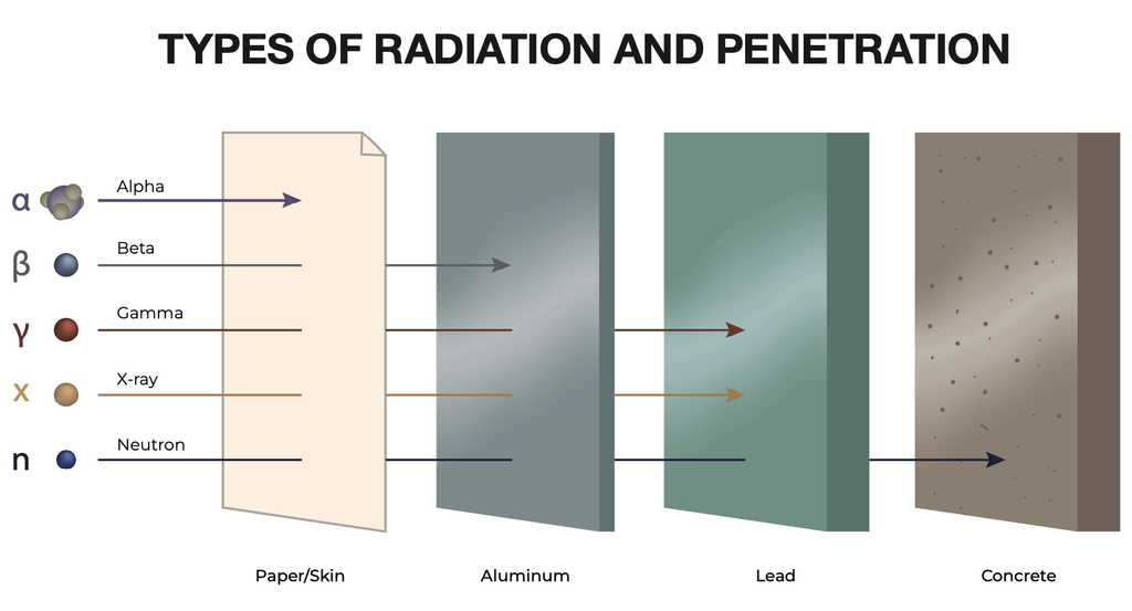
This leads us to radiation. Ansys Engineering describes radiation as the mechanism that transfers heat energy as electromagnetic waves or photons. That’s right, Capt. Kirk, that phaser technology might just be real! In other words, thermal energy can cause the atoms in any matter to move. The movement of those charged particles (protons and electrons at an atomic level) will result in the release of electromagnetic radiation. In its purest form, radiation heat transfer will only occur in a vacuum or through a medium that is transparent to the radiation. Furnace atmospheres come to mind.
Also, re-radiation is possible from an object, such as a heat treating load, so the radiant source is also absorbing radiation some of the time. Radiation transfer is very efficient and is used effectively in radiant tube furnaces. The tubes are heated electrically or by gas burners, and when they begin to glow (somewhere around 1250°F), they begin in earnest to try and bring the furnace or the load up to temperature.
Image Credit: Ashikul / AdobeStock
When radiation is at work, these types of heating devices provide good temperature uniformity. This is because once the furnace has determined that the chamber temp has been achieved, the radiation will continue to try to bring the chamber up to temperature, and these electromagnetic pulses try for equilibrium in the chamber.
Radiation is very efficient in most cases. Radiation is like a living thing — it wants everything to be the same temperature. So it normally has sight line between the glowing heat source and the load. Thermal radiation transfers heat via infrared rays and visible light waves. Hot furnace walls and heating elements emit these electromagnetic waves, which then heat the metal parts without needing direct contact or air movement.
That covers the styles and methods of heat transfer we can see in our heat treating shops. We’ll pick up a new topic next month.
About The Author:
Jim Roberts President US Ignition
Jim Roberts president at U.S. Ignition, began his 45-year career in the burner and heat recovery industry focused on heat treating specifically in 1979. He worked for and helped start up WB Combustion in Hales Corners, Wisconsin. In 1985 he joined Eclipse Engineering in Rockford, IL, specializing in heat treating-related combustion equipment/burners. Inducted into the American Gas Association’s Hall of Flame for service in training gas company field managers, Jim is a former president of MTI and has contributed to countless seminars on fuel reduction and combustion-related practices.
Inductor design plays a critical role in heating efficiency, temperature uniformity, and process stability, but conventional manufacturing methods can limit what coil geometries are possible. In this Technical Tuesday installment, Max Wissing, technology manager at PROTIQ, explores how 3D-printed copper inductors expand design freedom, allowing heat treaters to more closely tailor electromagnetic fields, cooling, and overall coil performance to demanding applications.
This informative piece was first released inHeat Treat Today’sOctober 2026 Ferrous & Nonferrous Heat Treatments/Mill Processing print edition.
Why Inductor Design Matters More Than Ever
Induction heating remains one of the most established and widely used technologies in modern heat treating. It enables precise, contactless energy transfer and offers a high degree of repeatability, making it particularly suitable for demanding applications, such as surface hardening, partial hardening, and localized treatment of highly stressed components.
At the same time, requirements in industrial heat treatment continue to increase. Manufacturers are expected to improve energy efficiency, reduce cycle times, and maintain consistent process quality. These demands are further intensified by the growing complexity of component geometries, which require more precise control of electromagnetic fields and temperature distribution than ever before.
Within this context, the inductor itself becomes a decisive factor, as its design directly influences heating behavior, efficiency, and process stability. However, many conventional inductors are still constrained by the limitations of their manufacturing methods. These constraints often force compromises between manufacturability and functional performance, meaning that coil geometries are not always ideally adapted to the component or the specific heat treat application. In more complex cases, this can lead to reduced energy efficiency or non-uniform temperature distributions, ultimately affecting process consistency.
In response, recent developments have increasingly focused on application-driven coil design and improved engineering approaches. Industrial 3D printing introduces a fundamentally different paradigm by enabling inductors to be designed according to functional requirements rather than production constraints. This shift opens up new possibilities for optimizing electromagnetic field distribution, improving energy transfer, and enhancing overall process performance in induction heat treating.
Where Conventional Coil Design Reaches Its Limits
Traditional induction coils are typically manufactured by bending and assembling copper tubes or machined elements. These methods are well established and widely used, but they impose inherent restrictions that can limit further optimization.
Geometric flexibility, for example, is constrained by bending radii and available tube profiles. As a result, the coil design often represents a compromise between what is theoretically optimal and what can be manufactured. In more complex applications, this can lead to non-uniform heating or less efficient energy coupling.
In addition, conventional manufacturing involves a considerable degree of manual work, which can introduce variability. Small deviations in geometry may affect electromagnetic behavior and, consequently, process consistency. The presence of joints — created through soldering or welding — further introduces potential weak points that can impact durability under thermal and mechanical stress.
Taken together, these factors not only influence manufacturing efficiency but also define the performance limits of the entire induction heating process.
3D Printing as a Design Enabler
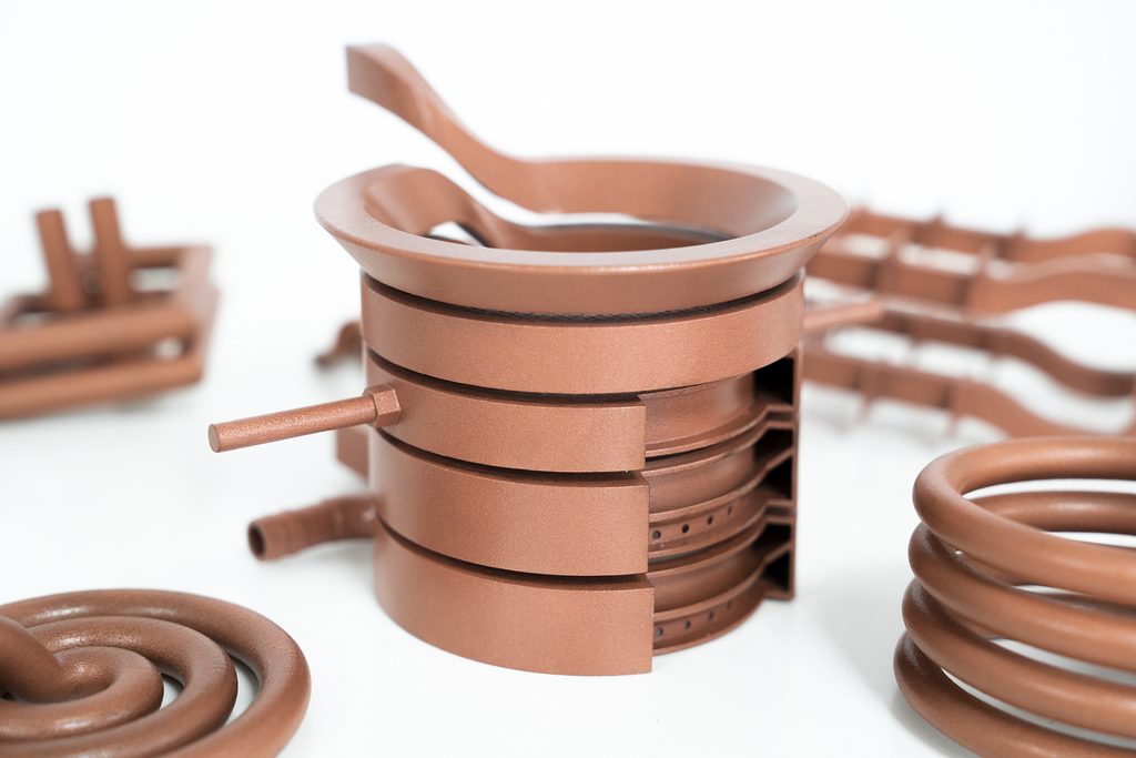
Industrial metal 3D printer | Image Credit: PROTIQ
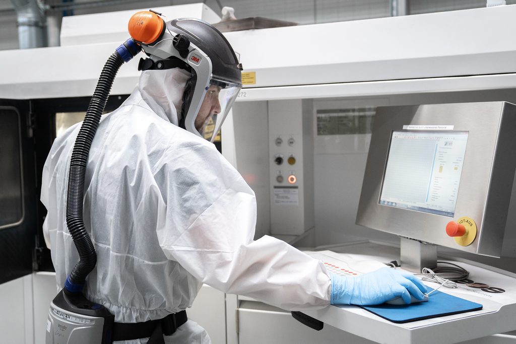
Additive manufacturing, often referred to as industrial 3D printing, is a production technology that creates metal components directly from digital design data. In processes like laser powder bed fusion (LPBF, often called SLM), a high-power laser selectively melts thin layers of metal powder. By repeating this process layer by layer, complex metal parts can be produced without the need for molds, tooling, or many of the manufacturing steps associated with conventional production methods.
This manufacturing approach offers a fundamentally different level of design freedom. Traditional manufacturing processes often require designers to adapt component geometries to machining, forming, or joining constraints. With additive manufacturing, many of these restrictions can be reduced or eliminated, allowing engineers to focus more directly on the functional requirements of the heat treatment application.
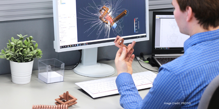
For induction heating, this means that the geometry of the inductor can be tailored more closely to the desired electromagnetic field distribution and heating characteristics. As a result, component design, process requirements, and performance objectives can be aligned more effectively.
Another important advantage is the ability to manufacture inductors as monolithic components. Instead of assembling multiple individual parts, the inductor can be produced in a single piece. This eliminates joints that may act as potential mechanical weak points while also enabling the integration of internal features, such as cooling channels. These channels can follow complex three-dimensional paths that would be difficult or impossible to realize with conventional manufacturing methods, enabling more targeted and efficient thermal management.
Impact on Induction Heating Performance
The increased design freedom enabled by additive manufacturing translates directly into improved process performance. When the geometry of the inductor is closely matched to the component, the electromagnetic field can be shaped more precisely. This allows for a more uniform temperature distribution, which is essential for achieving consistent material properties in heat treated parts.
Inductor with spray cooling | Image Credit: PROTIQ
Optimized geometries also improve the coupling of energy into the workpiece. In practical terms, this means that the required heating energy can be delivered more efficiently, often resulting in shorter cycle times. At the same time, improved cooling concepts help stabilize the process by keeping the inductor within its operating limits, even under demanding conditions.
Because additive manufacturing allows components to be reproduced with high accuracy, it also supports consistent process results. Compared to manually fabricated coils, this reproducibility reduces variability and contributes to overall process stability. The absence of soldered or welded joints can further increase service life, as common failure mechanisms are eliminated by design.
Copper in Additive Manufacturing: From Challenge to Application
Copper is the preferred material for induction coils due to its high electrical conductivity. However, its processing in laser-based additive manufacturing systems has long been considered challenging. The high reflectivity of copper and its thermal conductivity make it difficult to achieve stable and efficient melting during the build process.
In recent years, these challenges have been addressed through advances in machine technology, laser systems, and material development. Today, it is possible to manufacture copper components with properties suitable for demanding industrial applications, including conductivity levels comparable to conventional materials.
Despite this progress, successful implementation still requires a detailed understanding of both material behavior and process conditions. The interaction between geometry, material properties, and manufacturing parameters must be carefully considered to ensure that the final component meets both functional and mechanical requirements.
Companies such as PROTIQ have developed extensive experience in processing pure copper by additive manufacturing. This knowledge helps ensure stable production processes and application-oriented solutions for demanding industrial components like inductors.
Bridging Design and Reality Through Simulation and Experience
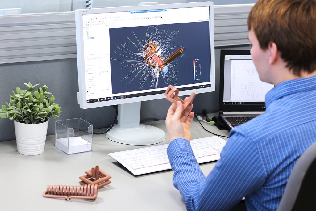
Simulation tools are an important element in the development of modern inductors. They provide insights into electromagnetic field distribution and thermal behavior, allowing engineers to evaluate and optimize designs before manufacturing.
However, simulation alone cannot fully predict how a component will perform under real operating conditions. Factors, such as material characteristics, surface quality, and manufacturing tolerances, can influence actual results. For this reason, experience in both additive manufacturing and induction applications remains essential.
In practice, effective inductor development is based on a combination of simulation, engineering expertise, and manufacturing know-how. This integrated approach helps ensure that theoretical designs can be translated into reliable solutions for industrial use.
Typical Applications in Heat Treating
The advantages of additively manufactured inductors become particularly evident in applications where conventional designs reach their limits. This is often the case in the heat treatment of components with complex geometries or varying cross-sections, where uniform heating is difficult to achieve.
In surface hardening processes, for example, tailored coil geometries can improve the consistency of hardness profiles across critical areas. Similarly, localized hardening applications benefit from the ability to precisely confine the electromagnetic field to specific regions of the component.
Another important field of application involves components with limited accessibility or intricate features. Here, additive manufacturing allows the realization of coil designs that can be adapted closely to the part geometry, enabling effective heating in areas that are difficult to reach with conventional inductors.
These application scenarios illustrate how additive manufacturing expands the solution space in induction heating, particularly for tasks that require a high degree of customization.
From Technology to Industrial Practice
While additive manufacturing offers significant opportunities, its successful use in induction heating depends on several factors. Material selection, manufacturability, and process stability must all be considered from the outset. Not every theoretically optimal design can be produced reliably, and design decisions must account for the specifics of the additive process.
Equally important is a deep understanding of the application itself. The requirements of the heat treat process, the properties of the component, and the desired outcomes must all be reflected in the inductor design.
In practice, additive manufacturing is not always the only or best solution. Depending on the application, a combination of conventionally manufactured and additively produced features can provide the most effective balance between performance, manufacturability, and cost.
This is where manufacturing expertise becomes critical. Companies like PROTIQ support clients in evaluating which parts of an inductor benefit from additive manufacturing and which may be better suited to conventional production methods. By combining process knowledge, material expertise, and industrial manufacturing capabilities, innovative designs can be translated into reliable and economically viable components.
Application-Driven Inductor Design
Additive manufacturing represents a shift in how induction coils are conceived and realized. By removing many of the constraints associated with conventional manufacturing, it enables a more direct alignment between design and function.
For heat treat operations, this opens up new possibilities for improving efficiency, quality, and reliability. Instead of adapting processes to the limitations of available coil geometries, inductors can be tailored to the specific requirements of the application.
As the technology continues to mature, additively manufactured inductors are likely to become an increasingly important element in advanced heat treat processes. Their successful application, however, depends not only on access to manufacturing technology but also on a comprehensive understanding of materials, processes, and application context.
About The Author:
Max Wissing Technology Manager PROTIQ
Max Wissing is the technology manager for 3D printing at PROTIQ with nearly a decade of industry experience. He holds a degree in mechanical engineering, specializing in the optimization of 3D-printed induction coils.
Ask The Heat Treat Doctor® has returned to bring sage advice to Heat Treat Today readers and to answer your questions about heat treating, brazing, sintering, and other types of thermal treatments as well as questions on metallurgy, equipment, and process-related issues. In this Technical Tuesday installment, Dan Herring explores practical guidelines for getting heat treatment right the first time, every time, in the first part of a series inspired by the work of Jon L. Dossett. He outlines seven keys to success in heat treating and the two questions design engineers must answer about what a component must endure in service and how it will be made. He then examines the most common specification mistakes, including unrealistic hardness, case depth, and tolerance requirements, and shows how carbon content, section size, mass effect, and commercially achievable tolerances determine whether a steel can be hardened to specification.
This informative piece was first released in Heat Treat Today’sSeptember 2026 People of Heat Treat print edition.
In our day-to-day work, most of us face the challenge of meeting production demands while navigating tight manufacturing deadlines in an ever-changing materials and manufacturing landscape. Heat treatment can be defined as the controlled application of time, temperature, and atmosphere to produce a predictable change in the internal structure (i.e., microstructure) of a material, resulting in the desired metallurgical, mechanical, physical, and other properties we desire. There is, however, an alternate and equally important definition of heat treating: getting the job done right the first time — every time.
In this short series, we will examine practical guidelines to help make that objective a reality. Let’s learn more.
7 Keys to Success in Heat Treating
To accomplish this goal, we must be able to meet the seven key considerations in heat treating to ensure both our success and survival (Herring 2014a, 2014b, 2015):
To know, metallurgically, what you want to accomplish.
To be able to predict the outcome of a heat treatment operation.
To have repeatability built into the process.
To get the most out of the equipment you have and to use state-of-the-art heat treating equipment whenever possible.
To be aware of how changes to our manufacturing operations influence the outcome of a given heat treatment process or series of processes.
To not compromise on quality.
To know our costs and understand our profitability.
Challenges Faced by Today’s Engineers
In the design of any engineered component, it is necessary to fully understand and address two key questions that design engineers working with metallurgists are often best qualified to answer (Herring 2014a, 2015, 2017):
What must the component endure during service (i.e., what are the product requirements)? To answer this question, consider the following: What are the rigors of the application, and what is the design life? Must the component part provide premier service, or is there an adequate design life involved (i.e., will other factors end its service long before its useful life is expended)? What loading, lubricants, temperature, and contaminants are involved? What other service and performance aspects specific to the product must also be factored into the selection process?
How will the component part be made (i.e., what are the process requirements)? Consider the following: How will its basic form be generated, and how will it be heat treated — if at all? Will it be important to introduce particular mechanical properties? If so, how (i.e., by heat treatment or by mechanical means)? Is geometry or surface finishes important? Will special coatings be used? Is dimensional control (including stability at temperature) an issue? What other processing aspects specific to the product must be considered?
How We Achieve Our Goals
Experienced heat treaters often point to the most common mistakes made by design engineers and/or their clients, that is, selecting materials, defining and understanding the limitations of the requested heat treatment processes, and specifying realistic outcomes from heat treating.
These include, for example, the desired hardness, case depth, and dimensional tolerances. These issues generally result from a failure to recognize the differences in the material’s chemical composition and form (e.g., wrought or powder metallurgy, castings, forgings). The design engineer should also understand the mill processing methods used to produce the material.
Often, the tolerances for the specified heat treatment properties are either too aggressive, too ambiguous, or too restrictive from a real-world standpoint. Here are a few basic metallurgical guidelines that can, from a practical standpoint, help avoid these problems (Herring 2014a, 2015; Dossett 2007, 2026).
Steel Selection
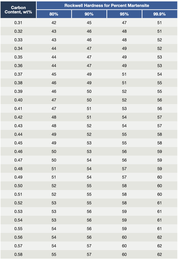
Table A. Carbon Content vs. Hardness for Different Martensite Levels (Dossett 2007)
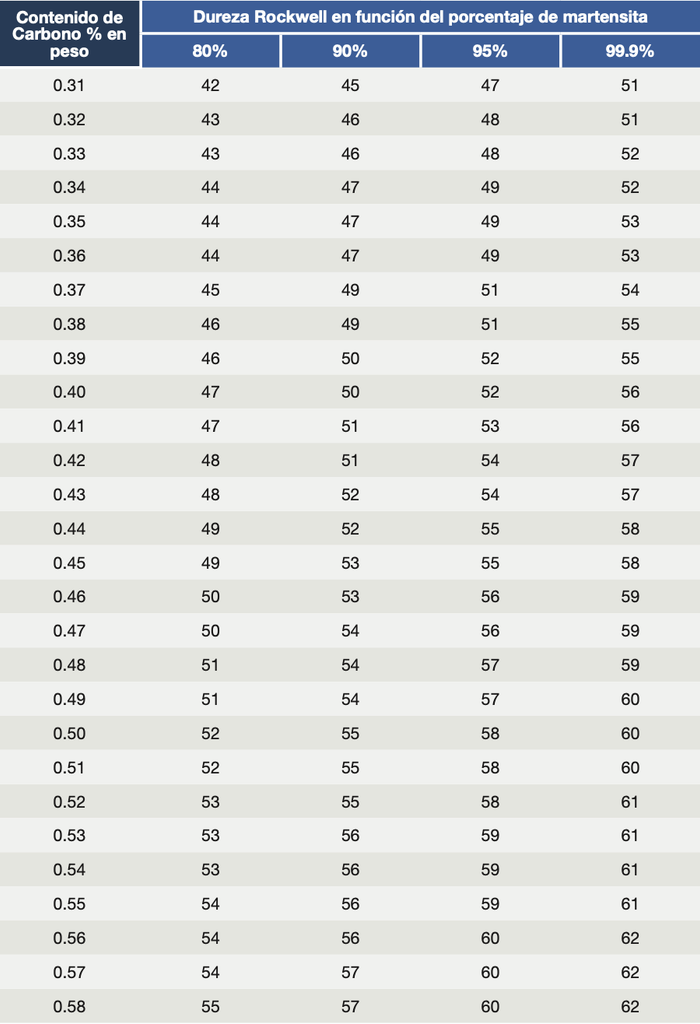
Problems in specifying the proper steel grade for a particular application generally involve choosing a steel grade that cannot be hardened to the specification and/or specifying a surface or core hardness range that is too restrictive. For example, Table A provides a guideline for the maximum surface hardness achievable using induction or flame hardening treatments. The maximum obtainable hardness is a function of the carbon content of the steel being used.
If the material selected is 4140H with a carbon range of 0.37–0.44%, we would expect the surface to be approximately 99.9% martensite after quenching. Thus, the expected as-quenched hardness would fall in the range of 54–58 HRC for all the heats of this steel. However, the ability to achieve this hardness depends on the severity of quenching, the quenchant used, the quench tank design, and the adequate removal of surface decarburization that might be present on the wrought steel itself.
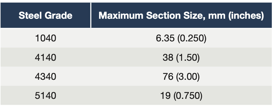
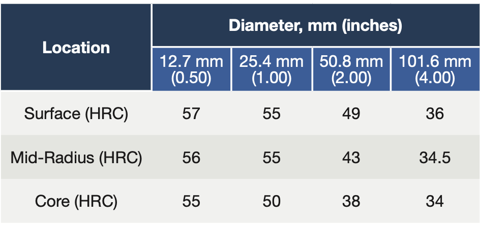
Table B. Maximum Surface Hardness as a Function of Section Size (Chandlar 1995)Table C. Mass Effect on Maximum Surface Hardness: (Oil) Quenched 4140 Steel (0.40%C) (Bethlehem Steel Company 1949)
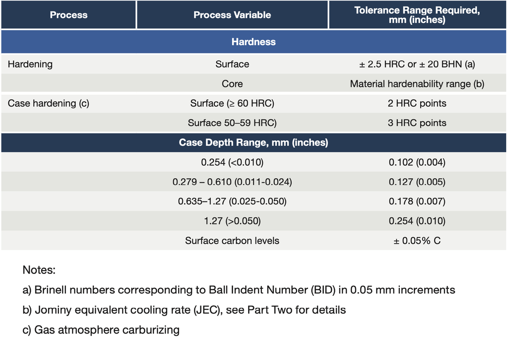
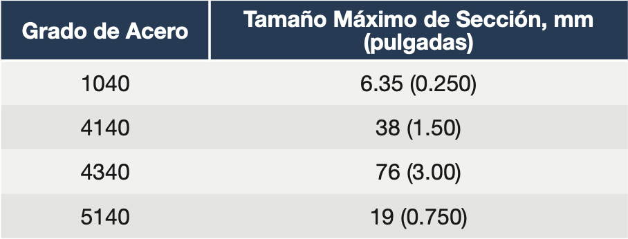
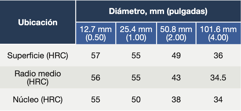
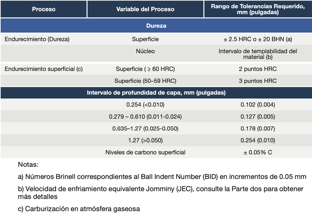
By contrast, in the case of furnace heat treatment, the maximum attainable surface hardness depends both on steel’s carbon content and its hardenability. The maximum section size (Table B) and effect of mass (Table C) are shown for several steel grades based on oil quenching. The commercially accepted range for surface hardness after tempering is ± 2.5 HRC points or ± 20 BHN points (Table D).
Table D. Commercially Desired Print Specification Tolerances for Properly Specified Materials
Next month we will review steel hardenability and how to determine the expected core hardness range.
This series was motivated by and contains insightful content from Jon L. Dossett who has granted permission. Jon’s distinguished career includes commercial heat treating involvement, extensive teaching career at ASM, and his work as editor of several volumes of the ASM Handbook series.
References
Bethlehem Steel Company. 1949. Modern Steels and Their Properties. Handbook 268. Bethlehem, PA: Bethlehem Steel Company.
Chandlar, Harry, ed. 1995. Heat Treater’s Guide: Practices and Procedures for Irons and Steels. Materials Park, OH: ASM International.
Dossett, Jon. 2007. “Make Sure Your Specified Heat Treatment Is Achievable.” Heat Treating Progress (March/April).
Dossett, Jon. 2025. Private conversation.
Herring, Daniel H. 2014a. Atmosphere Heat Treatment. Vol. 1. Troy, MI: BNP Media Group II.
Herring, Daniel H. 2014b. “Industry 4.0 and the 7 Key Considerations in Heat Treating.” Industrial Heating (September).
Herring, Daniel H. 2015. Atmosphere Heat Treatment. Vol. 2. Troy, MI: BNP Media Group II.
Herring, Daniel H. 2017. “The Relevance of Metallurgy in Engineering and Manufacturing.” Industrial Heating (November).
About the Author
Dan Herring “The Heat Treat Doctor®” The HERRING GROUP, Inc.
Dan Herring has been in the industry for over 50 years and has gained vast experience in fields that include materials science, engineering, metallurgy, new product research, and many other areas. He is the author of six books and over 700 technical articles.
Ask The Heat Treat Doctor® ha regresado para ofrecer consejos sabios a los lectores de Heat Treat Today y responder sus preguntas sobre tratamiento térmico, soldadura fuerte (brazing), sinterizado y otros tipos de tratamientos térmicos, así como preguntas sobre metalurgia, equipos y problemas relacionados con los procesos. En esta entrega de Technical Tuesday, Dan Herring explora lineamientos prácticos para lograr un tratamiento térmico correcto desde la primera vez, todas las veces, en la primera parte de una serie inspirada en el trabajo de Jon L. Dossett. Presenta siete claves para el éxito en el tratamiento térmico y las dos preguntas que los ingenieros de diseño deben responder sobre lo que un componente debe soportar en servicio y cómo se fabricará. Después examina los errores de especificación más comunes, entre ellos requisitos poco realistas de dureza, profundidad de capa y tolerancias, y muestra cómo el contenido de carbono, el tamaño de sección, el efecto de la masa y las tolerancias comercialmente alcanzables determinan si un acero puede endurecerse conforme a la especificación.
Este artículo informativo se publicó por primera vez en Heat Treat Today’sSeptember 2026 People of Heat Treat print edition.
Si tiene comentarios o preguntas sobre este artículo, háganoslo saber en: editor@heattreattoday.com.
En nuestro trabajo diario, la mayoría enfrentamos el desafío de cumplir con las demandas de producción mientras manejamos plazos de procesamiento ajustados en un panorama de materiales y manufactura en constante cambio. El tratamiento térmico puede definirse como la aplicación controlada de tiempo, temperatura y atmósfera para producir un cambio predecible en la estructura interna (es decir, la microestructura) de un material, dando como resultado las propiedades metalúrgicas, mecánicas, físicas y otras propiedades que deseamos. Sin embargo, existe una definición alterna e igualmente importante del tratamiento térmico: “hacer bien el trabajo desde la primera vez, todas las veces”.
En esta breve serie, examinaremos lineamientos prácticos para ayudar a hacer realidad ese objetivo. Conozcamos más.
7 claves para el éxito en el tratamiento térmico
Para alcanzar este objetivo, debemos ser capaces de cumplir con siete consideraciones clave del tratamiento térmico para asegurar tanto nuestro éxito como nuestra supervivencia (Herring 2014a, 2014b, 2015):
Saber, desde el punto de vista metalúrgico, lo que se desea lograr.
Ser capaz de predecir el resultado de una operación de tratamiento térmico.
Incorporar repetibilidad en el proceso.
Obtener el máximo provecho del equipo disponible y utilizar equipos de tratamiento térmico de última generación siempre que sea posible.
Ser conscientes de cómo los cambios en nuestras operaciones de manufactura influyen en el resultado de un proceso de tratamiento térmico determinado o de una serie de procesos.
No comprometer la calidad.
Conocer nuestros costos y comprender nuestra rentabilidad.
Desafíos que Enfrentan los Ingenieros de Hoy
En el diseño de cualquier componente de ingeniería, es necesario comprender plenamente y abordar dos preguntas clave que los ingenieros de diseño que trabajan con metalurgistas suelen estar mejor capacitados para responder (Herring 2014a, 2015, 2017):
¿Qué debe soportar el componente durante el servicio (es decir, ¿cuáles son los requisitos del producto?) Para responder esta pregunta, considere lo siguiente: ¿Cuáles son las exigencias de la aplicación y cuál es la vida útil del diseño? ¿Deberá el componente proporcionar un servicio de primera calidad o existe una vida útil de diseño adecuada (es decir, ¿otros factores pondrán fin a su servicio mucho antes de que se agote su vida útil?) ¿Qué cargas, lubricantes, temperaturas y contaminantes están involucrados? ¿Qué otros aspectos de servicio y desempeño específicos del producto también deben considerarse en el proceso de selección?
¿Cómo se fabricará el componente (es decir, ¿cuáles son los requisitos del proceso?) Considere lo siguiente: ¿Cómo se generará su forma básica y cómo se tratará térmicamente si es que se realizará un tratamiento térmico? ¿Será importante introducir propiedades mecánicas específicas? De ser así, ¿cómo? (es decir, ¿mediante tratamiento térmico o por medios mecánicos? ¿Es importante la geometría o los acabados superficiales? ¿Se utilizarán recubrimientos especiales? ¿Es importante el control dimensional (incluida la estabilidad a temperatura)? ¿Qué otros aspectos de procesamiento del producto deben considerarse?
Cómo Alcanzamos Nuestros Objetivos
Los especialistas experimentados en tratamiento térmico suelen señalar los errores más comunes cometidos por los ingenieros de diseño y/o sus clientes, es decir, la selección de materiales, la definición y comprensión de las limitaciones de los procesos de tratamiento térmico solicitados y la especificación de resultados realistas del tratamiento térmico. Estos incluyen, por ejemplo, la dureza deseada, la profundidad de capa y las tolerancias dimensionales. Estos problemas generalmente se deben a no reconocer las diferencias en la composición química y la forma del material (por ejemplo, material trabajado o pulvimetalurgia, piezas fundidas, piezas forjadas). El ingeniero de diseño también debe comprender los métodos de procesamiento en planta utilizados para producir el material. Con frecuencia, las tolerancias para las propiedades especificadas del tratamiento térmico son demasiado exigentes, demasiado ambiguas o restrictivas desde un punto de vista práctico. A continuación, se presentan algunos lineamientos metalúrgicos básicos que, desde un punto de vista práctico, pueden ayudar a evitar estos problemas (Herring 2014a, 2015; Dossett 2007, 2026).
Selección del acero
Tabla A. Contenido de carbono vs. Dureza para Diferentes Niveles de Martensita (Dossett 2007)
Los problemas al especificar el grado de acero adecuado para una aplicación particular generalmente implican elegir un grado de acero que no puede endurecerse conforme a la especificación y/o especificar un intervalo de dureza superficial o del núcleo demasiado restrictivo. Por ejemplo, la Tabla A proporciona una guía sobre la dureza superficial máxima que se puede alcanzar mediante tratamientos de endurecimiento por inducción o por flama. La dureza máxima que puede obtenerse depende del contenido de carbono del acero utilizado.
Si el material seleccionado es 4140H con un intervalo de carbono de 0.37-0.44%, esperaríamos que la superficie fuera aproximadamente 99.9% martensita después del temple. Por lo tanto, la dureza esperada en condición de temple estaría en el intervalo de 54-58 HRC para todas las coladas de este acero. Sin embargo, la capacidad de alcanzar esta dureza depende de la severidad del temple, el medio de temple utilizado, el diseño del tanque de temple y la eliminación adecuada de la descarburización superficial que pudiera estar presente en el propio acero trabajado.
Tabla B. Dureza superficial máxima en función del tamaño de sección (Chandlar 1995)Tabla C. Efecto de la masa sobre la dureza superficial máxima: acero 4140 (0.40%C) templado en aceite (Bethlehem Steel Company 1949)
Por el contrario, en el caso del tratamiento térmico en horno, la dureza superficial máxima alcanzable depende tanto del contenido de carbono del acero como de su templabilidad. El tamaño máximo de sección (Tabla B) y el efecto de la masa (Tabla C) se muestran para varios grados de acero templados en aceite. El intervalo comercialmente aceptado para la dureza superficial después del revenido es de ± 2.5 puntos HRC o ± 20 puntos BHN (Tabla D).
Tabla D. Tolerancias de especificación en plano comercialmente deseadas para materiales correctamente especificados
El próximo mes revisaremos la templabilidad del acero y cómo determinar el intervalo esperado de dureza del núcleo.
Esta serie surgió gracias a Jon L. Dossett, quien ha otorgado su autorización y contiene información valiosa aportada por él. La distinguida carrera de Jon incluye participación en el tratamiento térmico comercial, una extensa carrera docente en ASM y su trabajo como editor de varios volúmenes de la serie ASM Handbook.
Referencias
Bethlehem Steel Company. 1949. Modern Steels and Their Properties. Handbook 268. Bethlehem, PA: Bethlehem Steel Company.
Chandlar, Harry, ed. 1995. Heat Treater’s Guide: Practices and Procedures for Irons and Steels. Materials Park, OH: ASM International.
Dossett, Jon. 2007. “Make Sure Your Specified Heat Treatment Is Achievable.” Heat Treating Progress (March/April).
Dossett, Jon. 2025. Private conversation.
Herring, Daniel H. 2014a. Atmosphere Heat Treatment. Vol. 1. Troy, MI: BNP Media Group II.
Herring, Daniel H. 2014b. “Industry 4.0 and the 7 Key Considerations in Heat Treating.” Industrial Heating (September).
Herring, Daniel H. 2015. Atmosphere Heat Treatment. Vol. 2. Troy, MI: BNP Media Group II.
Herring, Daniel H. 2017. “The Relevance of Metallurgy in Engineering and Manufacturing.” Industrial Heating (November).
Acerca del Autor
Dan Herring “The Heat Treat Doctor®” The HERRING GROUP, Inc.
Dan Herring lleva más de 50 años en la industria y ha adquirido una vasta experiencia en áreas que incluyen ciencia de materiales, ingeniería, metalurgia, investigación de nuevos productos y muchas otras. Es autor de seis libros y de más de 700 artículos técnicos.
In this Technical Tuesday installment,Heat Treat Today founder and publisher Doug Glenn sat down with Steelhead Technologies CEO Jeff Halonen to discuss the company’s recent acquisitions of Visual Shop and Bluestreak. Learn what the acquisitions mean for current users, including support and migration timelines, and how Steelhead plans to bring decades of heat treat-specific expertise into its ERP platform.
Heat Treat Today founder and publisher Doug Glenn spoke with Steelhead Technologies CEO Jeffrey Halonen about the acquisitions and what commercial heat treaters can expect in the coming years.
The Companies and Their Software
Steelhead Technologies provides an all-in-one AI-powered ERP platform designed for job shops and manufacturing operations, connecting production management with quality, specification compliance and tracking, scheduling, accounting, CRM, reporting, and other business functions.
Halonen called Visual Shop one of the first commercially available systems built specifically for the heat treat market. Visual Shop has served process-oriented job shops for more than 30 years. Approximately 150 enterprises currently use Visual Shop, about half of which are commercial heat treaters. The ERP system was developed for metal finishing, heat treating, coatings, and related industries, with heat treat functionality including furnace-load tracking, specifications and certifications, process temperatures and times, order tracking, shipping, and invoicing.
Bluestreak has similarly deep roots in the industry. The QMS and MES platform was initially developed for heat treating and focuses on production workflow, integrated quality management, traceability, and compliance documentation. It has approximately 90 clients, about 60% of which are commercial heat treaters. “Bluestreak is a QMS and MES,” Halonen said. “They’re more specialized on the heat treating.”
The Acquisition Timeline
Although Steelhead acquired Visual Shop and Bluestreak within weeks of each other, Halonen said the deals developed separately, with different circumstances behind them and their timing largely coincidental. With Visual Shop, Halonen said the age and architecture of the software meant significant development would eventually require rebuilding the product. “It was just at a juncture where there’s either a tremendous amount of investment — many, many millions of dollars — to start from scratch, essentially, on a brand new product, or we could provide a structured transition over to a more modern system where there’s a definitive path,” he said.
Bluestreak, by comparison, was growing and had strong client retention. Retirement considerations for Bluestreak president and founder Todd Wenzel also played a role. Bluestreak also brings years of heat treat-specific software development, particularly around specifications, certifications, furnace compliance, and other quality requirements. “Bluestreak is on its fourth generation,” Halonen commented. “It’s been working with heat treaters for many, many years.”
Halonen acknowledged that the experience of these two software leaders in the space is important as Steelhead expands its presence in the heat treat industry. “Especially with commercial heat treating, there’s a tremendous amount of nuance,” he said. “We need to approach this with humility.”
Next Steps for Visual Shop and Bluestreak Clients
For existing clients, neither system is disappearing immediately. Visual Shop and Bluestreak are now under the Steelhead umbrella, but their existing support teams remain in place. “For Visual Shop, right now nothing changes,” Halonen said. “You have the same product, call the same exact team.”
The longer-term picture is different. Steelhead is targeting the end of 2027 for sunsetting support for Visual Shop. Many Visual Shop users have perpetual licenses, and Halonen emphasized that retiring support does not mean those users will suddenly lose access to the software. The primary change will involve continued support.
Bluestreak has a longer runway, with its timeline extending into 2028. Its existing support team also remains in place. At the same time, Steelhead intends to bring heat treat-specific functionality developed within Bluestreak into its own platform. “We’re working very closely as a single team to provide all the features that Bluestreak has developed over the years that are great for heat treaters and pulling those into Steelhead,” Halonen said.
One point is clear for users of both products: future software development will be focused on Steelhead’s technology. “All proactive R&D investment in technology is going into the Steelhead platform,” Halonen said.
Cost Considerations
For Visual Shop users considering a transition to Steelhead, price will be an important part of the decision. Halonen acknowledged that Steelhead carries a substantially higher software price.
Steelhead argues that shops should compare total operating costs rather than software prices alone, including separate accounting or business software and employee time associated with order entry, invoicing, and other administrative processes. “What we’ve found, though, is that if you look at the cost of operating your business on Visual Shop — not just the dollars you pay for Visual Shop — you actually see a cost reduction for Steelhead,” Halonen said. Whether that calculation holds true will depend on the individual operation. Heat treaters will need to weigh software costs against staffing, current processes, ancillary systems, desired functionality, and implementation requirements.
For Bluestreak users, Halonen said the pricing gap between their current system and Steelhead is smaller, although a difference remains.
Migration and Support
The acquisitions could simplify one challenge for clients who choose to migrate to Steelhead: transferring existing data. Steelhead now has access to the source code and database structures of the acquired platforms, as well as the employees familiar with them. “The data you have in Visual Shop and the data you have in Bluestreak can be mapped over in a much more efficient, and much more granular, manner than otherwise would be,” Halonen said.
The Visual Shop and Bluestreak teams — approximately eight and nine people, respectively — remain in place to support existing products and assist with integrations or migrations. Together with Steelhead’s roughly 310 existing clients, the acquisitions bring the company’s total client base to approximately 550.
Halonen said Steelhead also intends to control the pace of implementations rather than taking on migrations faster than its teams can support them. “If we’re in a position where we’re not 100% confident that it’s going to be successful for our client, we’re going to use the calendar to our advantage and make sure we’re not overscheduling or overburdening,” he said.
Where Development Goes from Here
Steelhead’s long-term strategy is to combine heat treat-specific knowledge from the acquired companies with its broader ERP platform. For Halonen, that starts with the fundamentals heat treaters rely on every day. “How can I do furnace calibrations? How can I create this certification? What’s my operator’s experience going to be?” he said, describing the questions heat treaters bring to Steelhead. “They’re absolutely correct to focus on that.”
Steelhead also plans continued development of automation and AI tools, including its existing AI-assisted order entry and analytics. But Halonen said those capabilities depend on getting the underlying systems right first. “None of that works unless you have a rock solid foundation,” he said.
What Heat Treaters Should Know Going Forward
The acquisitions do not require Visual Shop or Bluestreak users to make an immediate software change, but they do establish a clearer direction for both platforms. Visual Shop is targeted for end of life at the end of 2027, while Bluestreak’s timeline extends into 2028. Existing support remains in place, while future R&D is being directed toward Steelhead.
For affected heat treaters, that creates a window to evaluate their options. Which heat treat-specific capabilities are essential? What other systems or manual processes operate alongside the current software? What data must be preserved? What will implementation require from employees? And what will each option cost when software and business processes are considered together?
Three platforms are now under one company, and the software landscape serving heat treaters has shifted. The next couple of years give shops time to determine what that shift should mean for their own operations.
This article was written by Heat Treat Today’s Editorial Team.
Jim Roberts of U.S. Ignition engages readers in a Combustion Corner column about the modes of heat transfer at play in the heat treating world — breaking down advection and thermal conduction, from how forced air movement drives heating and cooling in furnaces to how Fourier’s law governs heat flow through direct contact, setting the stage for next month’s look at convection and radiation.
This editorial was first released in Heat Treat Today’sAugust 2026 Annual Automotive Heat Treating print edition.
A furnace guy walks into a heat treat facility and asks, “tropos metadosis thermotitas?” The furnace operators stare and say, “What are you saying? It’s all Greek to me!” But many of us know what it means: What mode of transfer? And that was the question of the last article where we looked at an intro to thermodynamics. This set us up for discussions on the four modes of heat transfer, a non-stop set of interactive processes that we then refine for our use in the heat treating world.
In that earlier discussion, we explained that there are several modes involved in heat transfer. Some are so simple to describe, but there may be several modes working at the same time to target the heat transference we seek. Modes of heat transfer and the Laws of Thermodynamics differ. Think of modes as the actual physical properties of heat transfer and thermodynamics that we can see and feel. The laws are the calculations and theory that allow us to check and produce the heat that is needed or to prove how much we need.
Our first mode of heat transfer is advection. Advection is the mechanism of thermal transfer that occurs when the thermal energy is transferred or transported from one space or object via the movement and the motion of a fluid. Pure convection, in the scientific sense, is strictly the heat transfer between heated bodies by gravitational lift or natural fluid movements.
In other words, heat rises… right? We’ve all heard it, witnessed it in a campfire or elsewhere. Advection is when the transfer media, mostly hot gases, is forced mechanically to swirl around and the item we desire to heat or cool. Speaking of heat transfer, we cannot forget that the door swings both ways. We can affect heat transfer from the standpoint of cooling things down too, and at that point, we discover that the hot gases or heat exchangers with air of liquid are using advection to pull the heat out. The plunge cool function of many furnaces relies on advection to pull the heat out of the parts at a controlled rate to cause a metallurgical change. So, the same laws apply, just in reverse!
One of the easiest ways to remember this difference is that advection actually adds energy to the process. It may be in the form of a blower providing combustion air for a burner, which creates the swirl of gases that are providing the heat transfer to the parts. Or, think of a fan pulling heat from a circuit board of electrical components. Advection is actually forced convection. If you have a modern convection oven or an air fryer, it is not really a convection oven. It’s an advection oven in the scientific world, since the fans involved are adding energy to move the fluid (air/gas) around those chicken wings and fries. The concern over this kind of added energy is in part what makes Data Centers such a volatile topic.
This leads us to our second heat transfer mode, thermal conduction. Thermal conduction is the transfer of heat by direct contact of two objects where there is a differential in temperature and energy. In other words, the temperature difference between two objects is the mechanism for heat transfer. Energy wants equilibrium, so it will always try to bring an item to its temperature by maintaining contact. It can be identified as thermal diffusion in Fourier’s law for heat conduction.
Fourier’s law states that eventually, through contact, the handle on the cooking pot will match the temperature of the pot surface because it is conducting the heat into that handle via thermal conduction. These types of considerations take place during calculations for furnace design, engine components, or household items; anything with a heat differential must be accounted for in our everyday lives.
As they say in the old country: choris thermotita, den yparchei ergo. Without heat, there is no work. That’s the loose translation, but it points out that we need to have all the components for heat transfer to be working for us to do this wonderful work called heat treating. And that shouldn’t be Greek to us.
Next month we will tackle convection and radiation.
About The Author:
Jim Roberts President US Ignition
Jim Roberts president at U.S. Ignition, began his 45-year career in the burner and heat recovery industry focused on heat treating specifically in 1979. He worked for and helped start up WB Combustion in Hales Corners, Wisconsin. In 1985 he joined Eclipse Engineering in Rockford, IL, specializing in heat treating-related combustion equipment/burners. Inducted into the American Gas Association’s Hall of Flame for service in training gas company field managers, Jim is a former president of MTI and has contributed to countless seminars on fuel reduction and combustion-related practices.
Heat Treat Today launches a new contributing experts series on emerging technologies reshaping heat treat operations. In this first installment, Zach Menard, CEO and co-founder of HRC Labs, demystifies deep neural networks (DNNs)— a technology quietly used in industrial settings for years — and explains how they turn accumulated furnace cycles, recipes, and quality records into predictive models that help heat treaters develop new recipes, minimize distortion, and cut cycle times.
This informative piece was first released in Heat Treat Today’sAugust 2026 Annual Automotive Heat Treating print edition.
Large language models (LLMs) have dominated recent conversations around artificial intelligence, but they are only one application of deep neural networks (DNNs). Years before DNNs were applied to human language, they had been deployed in industrial settings to optimize processes, improve yield, and support quality control.
These same, well-established approaches can be applied to heat treatment by learning relationships between process inputs — such as temperature, time, atmosphere, and alloy composition — and resultant metallurgical properties like hardness, distortion, or case depth.
It’s the first word in the acronym, DNN, that makes this learning possible. The neural network is said to be “deep” because of its many successive layers of neurons. Each neuron on its own is very simple. All it can do effectively is multiply and add together the numbers it has received from earlier neurons. However, when this process is repeated across many layers, the overall network is able to learn complex relationships that influence the heat treatment process.
By training on historical production data, DNNs can transform years of accumulated process knowledge into predictive models. Patterns that may otherwise remain buried across thousands of furnace cycles, recipes, and quality records can be captured quantitatively by the model itself.
In this way, operational experience and historical records become structured, reusable intelligence that can aid decision-making. Examples include when heat treaters are developing a new recipe, considering how to minimize distortion, or lowering cycle times.
As heat treatment operations continue accumulating larger volumes of process data, applying DNNs to this data offers a clear path toward AI-assisted process optimization, operational intelligence, and more adaptive heat treatment systems.
About the Author
Zachary Menard CEO and Co-Founder HRC Labs
Zachary (Zach) Menard is the CEO and co-founder of HRC Labs, an industrial AI company focused on process optimization and decision support for heat treatment. He holds a B.S. in physics from Vanderbilt University with a background in computational physics and machine learning research.
Ask The Heat Treat Doctor® has returned to bring sage advice to Heat Treat Today readers and to answer your questions about heat treating, brazing, sintering, and other types of thermal treatments as well as questions on metallurgy, equipment, and process-related issues. In this Technical Tuesday installment, Dan Herring explores the fundamentals of vacuum oil quenching — the three stages of oil quenching, the properties that make oil an effective quenching medium, and the ways pressure control, oil circulation, and temperature can be used to minimize part distortion — and offers step-by-step guidance on properly conditioning and degassing vacuum quench oil to ensure consistent, repeatable results.
This informative piece was first released in Heat Treat Today’sAugust 2026 Annual Automotive Heat Treating print edition.
Oil quenching in vacuum furnaces is a technology that has been around for over 65 years. The popularity of oil as a quench medium is due to its excellent performance and stability over a broad range of operating conditions. Proper application, testing, and conditioning of the oil are necessary to ensure its effectiveness. Let’s learn more.
For many, the choice of oil is not only due to metallurgical transformation and resultant properties it can achieve, but also to a number of other factors, including:
The first criterion that any quenchant must meet is its ability to approach an ideal quenching medium.
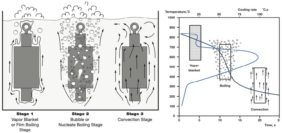
Figure 1a-b. Three stages of oil quenching
Regardless of the type of liquid (brine, water, polymer, oil, molten salt, or air mist), the ideal quenching medium (Figure 1) is one that would exhibit high initial quenching speed in the critical hardening range (Stages 1 and 2) and a slow final quenching speed through the lower temperature range (Stage 3). Thus, the ideal quenchant is one that exhibits little or no vapor blanket stage, a rapid but controlled nucleated boiling stage, and a slow cooling rate during convective cooling.
The high initial cooling rates allow for the development of full hardness by ensuring the steel misses the “nose” of the time-temperature-transformation diagram (i.e., quenching faster than the so-called critical transformation rate). This is followed by cooling at a slower rate beginning at the time the steel is forming martensite, which allows for better stress equalization so that the potential for distortion and cracking is reduced.
When conventional quenching oils are used, the duration of Stage 1 is longer, the cooling rate in Stage 2 is considerably slower, and the duration of Stage 3 is shorter. As such, the “quenching power” of oil is far less drastic than other quenchants. Water and water-based quenchants exhibit high initial cooling rates. Unfortunately, because of water’s low boiling point, this fast cooling persists until the steel is cooled to below 300°F (150°C). As most steels have formed or are forming martensite by this point, stresses are given little time to equalize. Thus, water is typically limited to low hardenability materials and relatively simple geometries.
Oil has a major advantage over water or polymer due to its higher boiling range. A typical oil has a boiling range between 450°F (230°C) and 900°F (480°C). This causes the slower convective cooling stage to start sooner, enabling the release of transformation stresses. Oil, therefore, is able to quench intricate shapes and high hardenability alloys successfully.
As it is heated, oil has a proportional drop in viscosity. This allows the quenchant to move more freely, increasing, in general, the tendency to break the vapor blanket layer. The nucleate boiling stage is not drastically altered by changes in bath temperature. The cooling rate in the convection stage, however, will slow as the bath temperature increases. This is advantageous for obtaining a slower rate of cooling through the austenite-to-martensite transformation range.
In general, as the temperature of a quenching oil increases, the overall quenching rate increases. Practical heat transfer coefficient (α) values are in the 1,000 to 2,500 W/m²K range depending on oil characteristics and degree of agitation. Peak α values are in the order of 4000 to 6000 W/m²K, or a cooling rate greater than 100°C/sec (180°F/sec).
Figure 2. Typical commercial heat treat load | Image Credit: The HERRING GROUP, Inc.Figure 3. Die cutting punches benefiting from controlling the pressure over the oil | Image Credit: The HERRING GROUP, Inc.
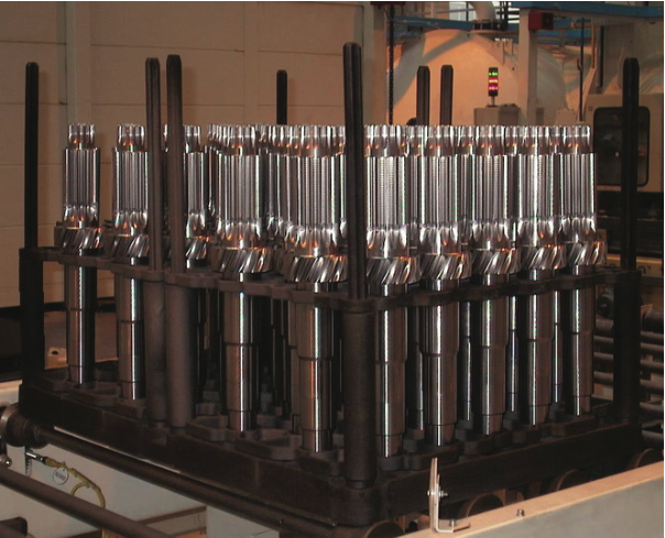
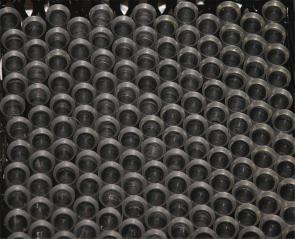
The use of vacuum oil quenching has been found to reduce distortion in many components including gears, pinions, and shafts (Figure 2). Oil quench vacuum systems also offer an attractive alternative to conventional atmosphere oil quenching, given their ability to vary a quench related variable not otherwise possible, namely controlling the pressure over the oil (Figure 3). This technique can be used to extend the range of part cross sections and materials that can be successfully hardened (Herring 1987, Sugiyama and Uchigaito 1987).
Pressure control along with oil temperature and oil circulation improves the predictability of distortion. The lower pressure allows for longer “vapor blanket” stages and a somewhat long “vapor transfer” stage, due to the reduced boiling point of the oil. This may reduce distortion and provide the desired hardness if the material’s transformation ranges are accommodating.
Distortion minimization methods have been used in combination with changes to flow characteristics. Some manufacturers pull oil down through the workload as opposed to pushing it upward. Also, oils formulated for vacuum service typically have a low vapor pressure, allowing them to be easily degassed.
Finally, vacuum systems do not permit the buildup of water in the quench tanks. In a vacuum furnace system, where vacuum is used to process the work or purge the quench environment, moisture will be removed as the system is evacuated and the oil circulated. Circulating the oil carries any moisture to the oil surface, where it vaporizes and is removed by the vacuum pumping system.
Maintaining Your Vacuum Quench Oil
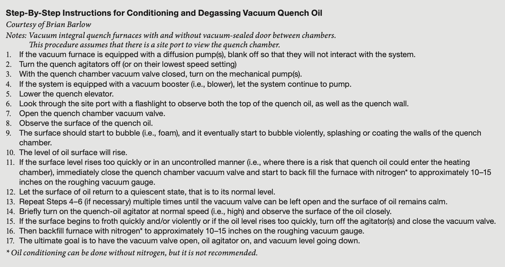
One of the aspects of vacuum oil quenching that is seldom documented is how to condition the quench oil. See “Step-By-Step Instructions for Conditioning and Degassing Vacuum Quench Oil” below.
Final Thoughts
As with all quenching, the key is to understand and control the key process variables. Proper selection of the type and use of oil under ideal conditions in a well-designed and well-maintained quench tank will ensure consistent and repeatable results.
Oil quenching should be applied in applications where its advantages outweigh its disadvantages and, as with all technologies, should be as completely understood as possible with respect to the performance requirements of the product so as to meet the application end use.
References
Brian Barlow. 2025. Private correspondence. Gasbarre Thermal Processing Solutions.
Herring, Daniel. H. 2002. “A Review of Factors Affecting Distortion in Quenching.” Heat Treating Progress Magazine. December. 2012. Vacuum Heat Treatment, Volumes I. BNP Media Group.
Herring, Daniel H. 2016. Vacuum Heat Treatment, Volume II. BNP Media Group.
Herring, Daniel H., Steven D. Balme. 2007. “Oil Quenching Technologies for Gears.” Gear Solutions. July.
Herring, D. H., Sugiyama, M., Uchigaito, M. 1986. “Vacuum Furnace Oil Quenching – Influence of Oil Surface Pressure on Steel Hardness and Distortion.” Industrial Heating Magazine. June.
Sugiyama, M., Uchigaito, M. 1987. “Controlling Oil Surface Pressure in Vacuum Oil Quenching.” Heat Treating Magazine. July.
About the Author
Dan Herring “The Heat Treat Doctor®” The HERRING GROUP, Inc.
Dan Herring has been in the industry for over 50 years and has gained vast experience in fields that include materials science, engineering, metallurgy, new product research, and many other areas. He is the author of six books and over 700 technical articles.
Ask The Heat Treat Doctor® has returned to bring sage advice to Heat Treat Today readers and to answer your questions about heat treating, brazing, sintering, and other types of thermal treatments as well as questions on metallurgy, equipment, and process-related issues. In this installment, Dan Herring explores the optimal dew point for running an endothermic gas generator — comparing the low dew point practices of decades past with today’s modern operating range of +40°F to +45°F — and explains how dew point, temperature, and air/gas ratio affect catalyst life, generator maintenance, and the stability of the process gas.
This informative piece was first released in Heat Treat Today’sJuly 2026 Annual Super Brands Issue print edition.
A critical consideration in heat treatment is the type, consistency, and control of the furnace atmosphere. The purpose of a furnace atmosphere varies with the desired end result, so it begs the question if there is an optimal dew point to operate an endothermic gas generator to balance gas quality, performance, and maintenance life. Let’s learn more.
Purpose of an Endothermic Gas Atmosphere
In general, furnace atmospheres are used:
To protect the components being processed from chemical reactions that could occur on their surfaces (e.g., oxidation or carburization), that is, to be passive (chemically inert) to the metal surface.
To interact with the surface of the component (e.g., adding carbon, or nitrogen, or both), that is, to be reactive (chemically active) to the metal surface.
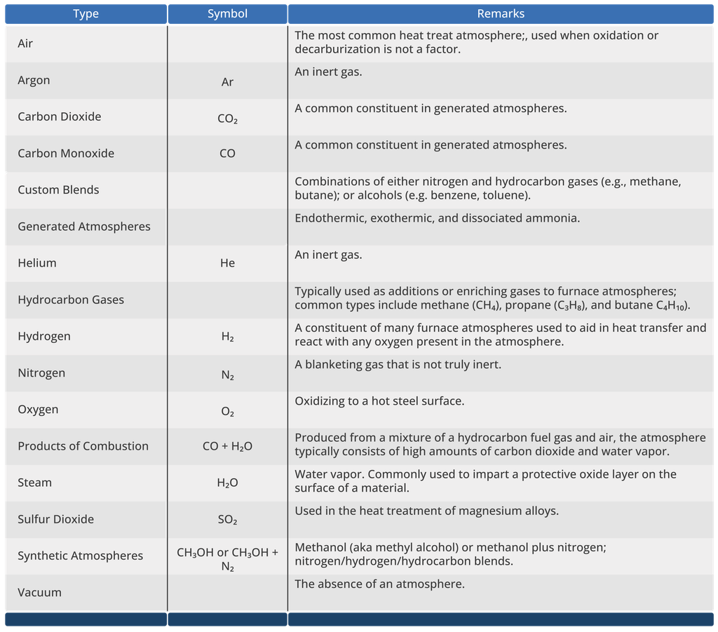
Table A. Common Types of Furnace Atmospheres
There are many types of furnace atmospheres available for use in heat treating (Table A). By far, one of the most common is endothermic gas.
Endothermic Gas Atmospheres
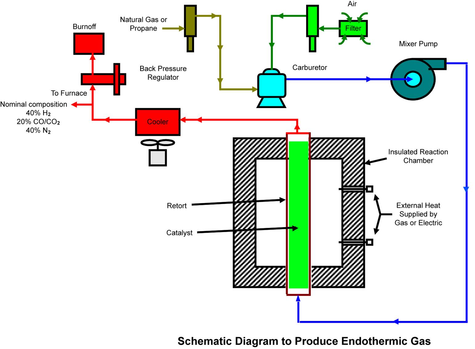
Figure 1. Endothermic gas generator schematic piping arrangement | Image Credit: The HERRING Group, Inc.
Endothermic gas generators are common equipment in the heat treat shop, with one of the most well-known generators being the RX®. The main components of an endothermic gas generator (Figure 1) are relatively simple, consisting of:
Heated reaction retort with catalyst
Air-gas proportioning control components
Pump to pass the air-gas mixture through the retort
Cooler to “freeze” the reaction and prevent soot formation
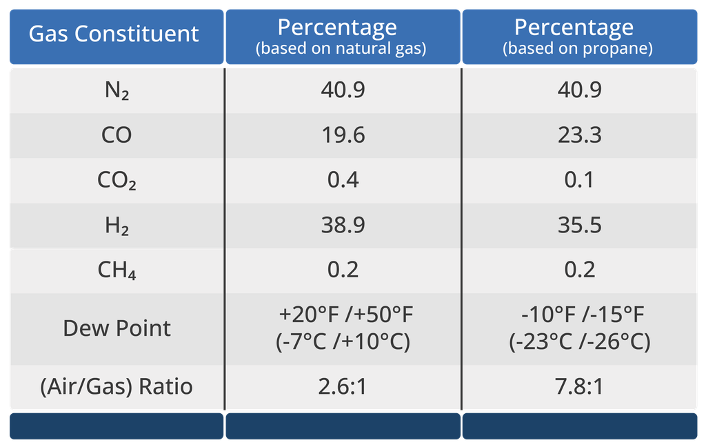
Table B. Compositional Ranges for Endothermic Gas
Endothermic gas (aka endo) is produced when a mixture of air and fuel is introduced into an externally heated retort at such a sufficiently low air-to-gas ratio that it will normally not burn. The retort contains an active catalyst, which aids in cracking the mixture. Leaving the retort, the gas is cooled rapidly to avoid carbon reformation (in the form of soot) before it is sent to the furnace. The endothermic gas composition (Table B), by volume, varies depending on the type of hydrocarbon gas feed stock.
Endothermic gas is typically used for applications such as neutral hardening gas carburizing and carbonitriding (as a carrier gas), and for certain types of brazing to name a few. It is generally produced so that its composition is chemically inert to the surface of the steel and can be made chemically active by the addition of enrichment (hydrocarbon) gas that is usually added at the furnace.
What is the Optimal Generator Dew Point?
A reader asked this important question: “I’m doing some searching on endothermic gas generation and the advantages/disadvantages of low/high dew point set points. We normally run a dew point of +50°F in our generator and have had success historically. We installed a new generator and were told to drop the dew point to +40°F as this would extend the life. Do you have any experience, or can you point me to any references listing some of the pros and cons of running lower and higher dew points?”
Past Thinking
The operating philosophy in yesterday’s heat treat shop was to run the generators at a low dew point, typically in the range of +30°F to +35°F, so that gas (or air) additions at the furnace could be minimized. The belief was that the furnace atmosphere was much more responsive at this range and controlling certain processes (e.g., carburizing) was easier.
The nickel content of the catalyst years ago varied by manufacturer but was typically in the 5–7.5% range. Given the operating parameters used, it was mandatory to run weekly air burnout cycles to minimize soot formation in the catalyst bed, which took place quickly at these low dew points. The catalyst also needed to be changed on average about every 12 months. This dew point range was considered a good compromise for heat treat shops that ran both carburizing and neutral hardening.
As a parenthetical note, the very first endothermic gas generators (which were charcoal fired) used 100% nickel balls as a catalyst.
Current Thinking
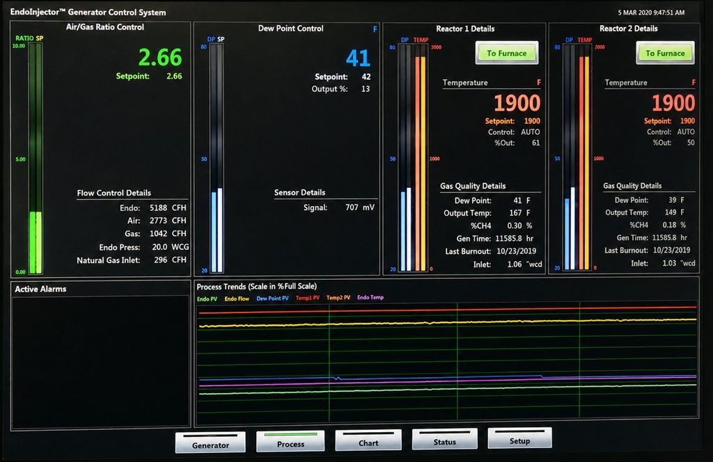
Today, and for roughly the last 20+ years, the “modern” thinking is to run endothermic gas generators at temperatures in the range of 1900°F–2000°F, depending on the manufacturer’s design and the materials and size (diameter and length) of the retort. Air/gas ratios (for natural gas) should be between 2.5:1 to 3.5:1 (Figure 2). Ratios as low as 2.0:1 can be run at higher generator operating temperatures. Gas and/or air additions are then done at the furnace for better process control.
Figure 2. Typical endothermic gas generator control panel | Image Credit: The HERRING Group, Inc.
Experience has shown that a generator running at 1900°F with an air gas ratio between 3.0:1 and 3.5:1 and an output dewpoint of +42°F provides the best combination of a stable process gas and maximum generator life.
A generator dew point range held between +40°F and +45°F reduces maintenance on the generator and decreases the frequency of performing air burnouts of the catalyst bed, which at these dew points only needs to be done approximately once a month. It also extends the life of the catalyst (upwards of 2+ years) and makes it easier for the modern controls to regulate the system. Remember, however, that gas transmission from the generator to the furnace can often raise the incoming furnace dew point by +5°F to +10°F.
The advantage of performing air burnouts less often is that the nickel coated catalyst lasts longer. A major reason for this is that today’s catalyst averages around 3% nickel. The catalyst is insulating firebrick dipped in a nickel sulfate bath to allow nickel absorption on the outer surfaces of the cubes or spheres.
Miscellaneous Remarks
One must be very careful when running dew points at +50°F or above. In the writer’s experience, the gas is much more unstable, the water (moisture) content of the gas can rise quicker than one might anticipate, and you can literally start “raining water” inside the furnace or in the transmission lines. In literally minutes, the endo dew point can rise from +50°F to +70°F if one is not careful.
In Summary
The subject of endothermic gas generators never grows old. The key to their success is finding an operating dew point that provides both a stable process gas and little maintenance downtime. However, planned preventative maintenance is still required and should be performed on a schedule determined by the number and type of problems that arise.
A future column will discuss specifics of generator control, and we will broaden the subject by providing a guideline to the selection of furnace atmospheres in heat treating, brazing, and sintering. Look for it in next month’s publication.
References
Herring, Daniel H. 2015. Atmosphere Heat Treatment, Volume II, BNP Media Group.
Herring, Daniel H. 2009. “Furnace Atmosphere Considerations During Heat Treating”, Furnaces International, March/April.
Herring, Daniel H. “Understanding Furnace Atmospheres, Atmosphere Operation and Atmosphere Safety,” Heat Treating Hints, Vol. 1 No. 7. Manuscript forthcoming.
About the Author
Dan Herring “The Heat Treat Doctor®” The HERRING GROUP, Inc.
Dan Herring has been in the industry for over 50 years and has gained vast experience in fields that include materials science, engineering, metallurgy, new product research, and many other areas. He is the author of six books and over 700 technical articles.
Machine learning is poised to become a powerful tool for modern heat treatment, transforming decades of production data into actionable process intelligence. In this Technical Tuesday installment, Zachary C. Menard, CEO and co-founder of HRC Labs, draws on real-world case studies in carburizing and tempering to explore how predictive models can accelerate recipe development, optimize operations, and support more consistent decision-making. Rather than replacing metallurgical expertise, data-driven tools offer a pathway to continuous improvement, greater efficiency, and stronger competitive advantage.
This informative piece was first released inHeat Treat Today’sJuly 2026 Annual Super Brands Issue print edition.
Introduction
Heat treatment is one of the most operationally demanding and variable processes in modern manufacturing. It operates at the critical intersection of process design, material variability, and the strict performance requirements of industries as diverse as automotive, aerospace, and construction.
As a result, even highly experienced heat treaters must routinely make high-stakes decisions: how to converge on a new recipe without expensive trial-and-error; how to increase throughput without sacrificing quality; and whether a deviation warrants rework or scrap.
Heat treaters are uniquely positioned to benefit from advances in machine learning when confronting these decisions. Years of archived process data, hardness measurements, and quality records represent a largely untapped resource.
When systematically modeled, this data can power predictive models that map recipe parameters to metallurgical outcomes.
This approach is not without precedent. Similarly complex industrial processes — aggregates mining, cement manufacturing, and even steel casting — have increasingly adopted machine learning to reduce variability, optimize cycles, and proactively detect process drift. These gains have not replaced domain expertise; they have amplified it.
The following sections outline how machine learning, when thoughtfully integrated with metallurgical understanding and domain expertise, can serve as an enabling infrastructure for modern heat treatment.
What is Machine Learning?
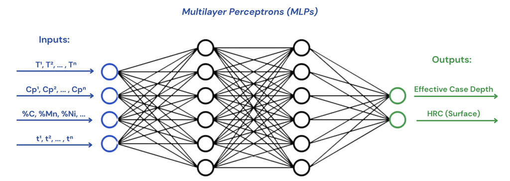
Machine learning (ML) refers to computer algorithms designed to learn how a system behaves by leveraging that system’s data. Among the most relevant ML models for heat treatment are multilayer perceptrons (MLPs), which are designed to learn complex, nonlinear relationships between process inputs and observed outcomes.
Image Credit: HRC Labs
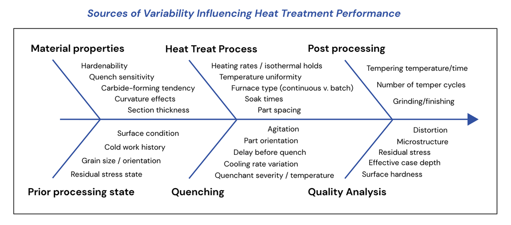
In heat treatment, outcomes such as surface hardness, effective case depth, distortion, or residual stress do not depend on any single variable. They emerge from the simultaneous interactions between variables like temperature, time, atmosphere composition, material composition, part geometry, and quench severity and uniformity, to name a few.
MLPs are well suited to modeling precisely this type of behavior. Rather than assuming a predefined relationship or physical law, they learn the mapping from process parameters to measured outcomes directly from historical production data. Layer by layer, the model captures increasingly subtle interactions among variables, enabling it to represent effects that are difficult to express with predetermined equations.
Importantly, once trained on sufficiently representative data, MLPs can:
Predict part properties for proposed recipes in milliseconds.
Evaluate hundreds of candidate parameter combinations rapidly.
Provide explicit uncertainty estimates alongside predictions.
Be tuned to individual furnaces, load configurations, or heat treatment techniques.
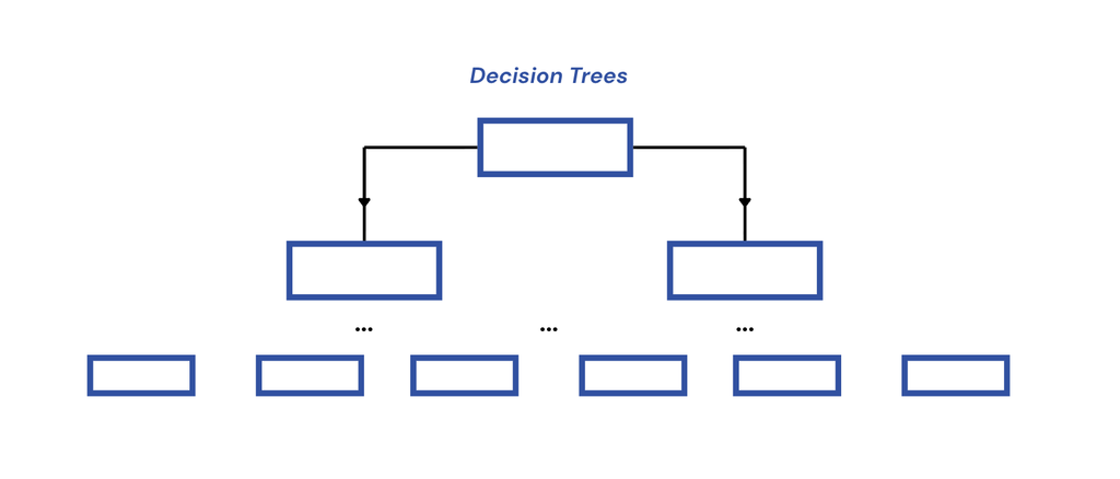
While MLPs are well suited to modeling the complexity of the heat treatment process, another class of machine learning models called decision trees are particularly effective for structured operational decisions. Heat treatment routinely requires categorical judgments, from rework decisions to detecting process drift to root cause analysis.
Decision trees can categorize heat treatment runs based on how they differ from historical runs. For example, the tree may organize a run based on its temperature deviations, fluctuations in carbon potential, or variation in effective case depth from the average. Each terminal node or “leaf” of the tree represents a cluster of historically similar runs.
Because these clusters are associated with prior corrective actions and results, the tree can provide probabilistic guidance grounded in historical precedent. For example, when analyzing a recent batch of parts that missed their target case depth, the tree might find that among comparable historical runs, 80% were successfully re-processed under a modified cycle, while 20% were scrapped. This enables faster root cause analysis and supports decision making.
Heat Treatment Applications
ML is particularly well suited to modeling and managing the many interacting variables that determine heat treatment outcomes. These capabilities translate into three practical applications: recipe development, process optimization, and auxiliary decision support.
Recipe Development
Heat treaters rely on operational experience, test coupons, and simulation tools to inform recipe design. However, new alloys, part geometries, or throughput demands often require iterative trial runs. Each additional load dedicated to experimentation represents furnace time removed from production.
Finite element simulations can narrow candidate recipes, but their accuracy depends on material properties, boundary conditions, and calibration to production conditions.
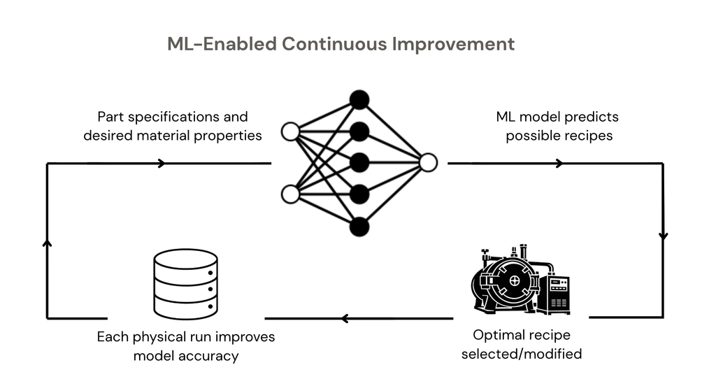
ML models such as MLPs offer a complementary approach to physical simulations. Trained on historical production data, they learn how a specific furnace, material, and process behave under real production conditions. Once trained, these models can rapidly evaluate candidate recipes against hardness, case depth, and distortion targets.
Importantly, predictions can be accompanied by uncertainty estimates, allowing heat treaters to assess risk alongside expected performance. By reducing the number of physical trial runs required to converge on a robust recipe, ML can accelerate the path from testing to production while preserving metallurgical oversight.
Process Optimization
Once a recipe has been demonstrated to meet specification, the focus shifts from feasibility to efficiency and robustness. The objective becomes reducing cycle time and energy consumption while maintaining process stability and required part properties.
In practice, optimization often proceeds through incremental parameter adjustments informed by experience. Soak times may be shortened or quench conditions modified in pursuit of efficiency gains. Yet the interdependence of heat treatment parameters makes it difficult to predict how such changes will affect process robustness.
ML models provide a structured framework for navigating this landscape. Once trained, they can:
Evaluate a multitude of potential changes to a recipe.
Estimate the impact of efficiency-driven adjustments on final properties.
Quantify uncertainty, identifying parameter sets that are not only efficient but stable.
Rather than relying solely on sequential physical trials, heat treaters can assess proposed modifications computationally before allocating furnace capacity.
Each additional production run further refines the model. As data accumulate across varying materials, geometries, and operating conditions, predictive fidelity improves. Over time, optimization transitions from periodic study to continuous, data-driven improvement.
Auxiliary Decision Support
Recipe design and optimization are only part of the operational challenge in heat treatment. A substantial portion of heat treaters’ time is devoted to diagnosing deviations, determining appropriate corrective action, and monitoring for process drift.
When a batch fails to meet specification, multiple correlated factors may plausibly explain the deviation. As a result, root cause analysis often requires time-consuming review of process logs and historical records.
Image Credit: HRC Labs
Decision-tree-based models provide a structured method for accelerating this analysis. By learning from historical runs and their documented outcomes, the model can classify a new deviation according to its similarity to past cases. For example, the model may determine that comparable historical runs were most frequently associated with temperature non-uniformity rather than alternative causes.
This approach offers three practical advantages:
Image Credit: HRC Labs
Faster root cause analysis and reduced diagnostic downtime.
More consistent, data-backed rework decisions.
Earlier detection of process drift and emerging equipment issues.
Importantly, these models do not override heat treaters’ judgment. Rather, they surface structured historical context that may otherwise remain fragmented across logs and institutional memory. Over time, this improves consistency, auditability, and knowledge transfer.
Machine Learning in Heat Treatment
The preceding sections have outlined several proposed applications of ML in heat treatment. The following sections examine documented cases of successful ML application in heat treatment.
Case Study 1: Carburizing
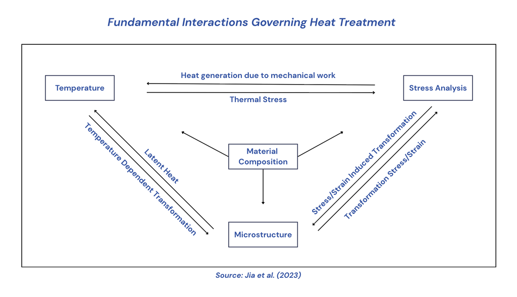
Jia et al. (2023) demonstrated the use of multilayer perceptrons to model the vacuum carburizing process for a low-alloy carbon steel cylinder. Using primarily simulation-derived data supplemented by limited experimental runs, the authors trained an MLP to predict case depth, surface carbon concentration, and surface hardness from process parameters including carburizing and diffusion temperatures, cycle durations, and carbon concentration levels.
Image Credit: HRC Labs
Once trained, the model rapidly identified parameter combinations that satisfied specified hardness and case depth targets while reducing computational cost relative to traditional simulation tools.
Zhang et al. (2025) took a similar approach but focused on atmospheric carburizing. The study’s goal was to train an MLP to predict post-carburizing carbon concentration across multiple part geometries for SAE AISI 3316 gear steel. Representative test coupons were used to validate the simulation-derived training data against production runs.
The model predicted post-carburizing carbon concentration with average errors near 2%. While limited in scope, both studies demonstrate that ML can replicate complex diffusion-driven behavior and accelerate recipe evaluation. These investigations focused primarily on carbon concentration and hardness prediction; the same modeling frameworks could be extended to distortion and residual stress prediction.
Case Study 2: Tempering
To further explore the performance of ML in heat treatment, publicly available tempering data from the classic study of Hollomon and Jaffe (1945) were analyzed. Their model combines temperature and time into a single tempering severity parameter, M. While effective within specific steels, prediction errors increased substantially as carbon contents varied. This model failed in particular to extrapolate to the behavior of lower carbon steels, with errors surpassing 10 HRC in some cases.
Image Credit: HRC Labs
To address this limitation, ML was used as a corrective layer on top of the traditional Hollomon-Jaffe model. The Hollomon-Jaffe equation provided baseline hardness predictions, while the ML model learned systematic corrections based on alloy composition and processing conditions. This approach reduced prediction error dramatically — from over 10 HRC in some cases to 2 HRC — while preserving the underlying metallurgical framework.
A common concern with ML models is that they behave like “black boxes.” However, modern interpretability tools allow engineers to examine how models arrive at their predictions. In this study, SHAP (SHapley Additive exPlanations) analysis was used to examine how the model corrected the Hollomon-Jaffe prediction. This revealed clear trends in how quantities like carbon concentration informed the model’s corrections. Rather than behaving like a black box, the model learned consistent metallurgical patterns in the data.
This case study illustrates how ML models can improve traditional approaches when they are limited by assumptions about physical parameters or cannot accommodate certain inputs. Unique furnace behavior, fixturing configurations, and part processing history are difficult to capture and calibrate using traditional simulation tools. Additional work should explore the integration of ML as a corrective layer for simulation software.
Strategic Implications and Competitive Advantage
The case studies presented here illustrate a broader principle: ML is most powerful in heat treatment not as a replacement for metallurgical understanding, but as a mechanism for formalizing and extending it.
When applied thoughtfully, ML can accelerate recipe development, reduce trial-and-error, and support structured diagnostics grounded in historical precedent. Unlike static optimization studies, trained models improve continuously as new production data become available. Over time, they become increasingly plant-specific, capturing nuances in furnace behavior, fixturing, material sourcing, and operating conditions that are difficult to encode with predefined equations.
Successful implementation will require high-quality process data and close collaboration between heat treaters and data scientists. ML is not a substitute for metallurgical expertise, but a tool for extending it.
The opportunity is substantial. Heat treatment has generated decades of process data that remain underutilized. Shops that convert this historical record into predictive intelligence will gain measurable advantages in efficiency, robustness, and process consistency. As competitive pressures increase and tolerances tighten, the ability to continuously learn from operations may become a defining differentiator.
Heat treatment has a rich history of innovation and experimentation. The integration of ML represents the next step in that progression.
Acknowledgements: The author would like to thank Dan Herring, The Heat Treat Doctor®, whose insight and guidance were instrumental in refining the direction of this work.
References
Hollomon, J. H., and L. D. Jaffe. 1945. “Time-Temperature Relations in Tempering Steel.” Transactions of the American Institute of Mining and Metallurgical Engineers 162: 223–49.
Jia, Hongliang, Dong Ju, and Jian Cao. 2023. “Machine Learning Based Optimization Method for Vacuum Carburizing Process and Its Application.” Journal of Materials Informatics 3: 9. https://doi.org/10.20517/jmi.2022.43.
Zhang, Y., Z. Tang, Q. Yin, et al. 2025. “Machine Learning Based Prediction of Carbon Concentration in Carburized Steel.” Scientific Reports 15: 33678. https://doi.org/10.1038/s41598-025-18531-8.
About The Author:
Zachary Menard CEO and Co-Founder HRC Labs
Zachary (Zach) Menard is the CEO and co-founder of HRC Labs, an industrial AI company focused on process optimization and decision support for heat treatment. He holds a B.S. in physics from Vanderbilt University with a background in computational physics and machine learning research.