Heat Treat Radio #131: Beyond Calibration — Real-World Accuracy in Heat Treat Measurement
What does it really take to achieve accurate temperature measurement in the real heat treat production? In this episode of Heat Treat Radio, host Heather Falcone sits down with Dr. Steve Offley, product marketing manager at PhoenixTM, to explore the science behind thru-process monitoring, thermal barriers, and data logger performance. From cold junction compensation to real-world shop floor challenges, they unpack why lab accuracy doesn’t always translate to production — and what heat treaters can do about it. Tune in to learn how to ensure your temperature data is as reliable as the parts you produce.
Below, you can watch the video, listen to the podcast by clicking on the audio play button, or read an edited transcript.


The following transcript has been edited for your reading enjoyment.
Introduction (00:04)
Heather Falcone: Today we are talking about a feature article coming up in this month’s magazine, Achieving Accurate Measurements in Real Heat Treat Production. Joining me today is author of this piece, Dr. Steve Offley from PhoenixTM, who is also our sponsor for today’s episode.

Steve is a product marketing manager at PhoenixTM with responsibility for both strategic product management and global marketing of the company’s thru-process temperature, optical profiling, and TUS system product range. Steve joined PhoenixTM in April of 2018 after 22 years of experience in the industrial temperature profiling market with another well-known company.
The Role of PhoenixTM (2:35)
Heather Falcone: Tell us about your role at PhoenixTM and the role of PhoenixTM, specifically how they provide solutions for the thermal processors out there.
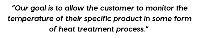
Steve Offley: I am the product marketing manager or product manager for the range of temperature monitoring systems that we offer to the wider industrial space. We provide support for clients in a range of industries who are faced with the daily challenges of using thermal processing as part of their key manufacturing step. We offer unique solutions for those specific applications, because not every application is the same. Our goal is to allow the customer to monitor the temperature of their specific product in some form of heat treatment process.
For instance, we could be offering a solution for the coating market, where a client wants to monitor the thermal cure of a car body. They want to ensure that that car body, as it travels through the curing oven, is achieving the correct temperature, not just in the oven itself, but at the product level. So is each part of that car body achieving the right temperature for the right duration to cure the paint?
Another day we might be dealing with a food processor who, as you can imagine, when they’re dealing with food safety and HACCP requirements, they want to prove that the core of their product, which may be a chicken fillet in a deep fat fryer, is achieving the right temperature, to make sure that it’s safe and it’s an attractive product to eat. And of course, they want to be confident that the consumer is going to be healthy after consuming the product too.
In the buildings and ceramics industry, for instance, we can offer the same sort of solution for the manufacturers of bricks, building materials, tiles, etc., where the process may actually be up to three or four days long where they’re drying the products. But it’s still critical to know what the temperature is at the product level.
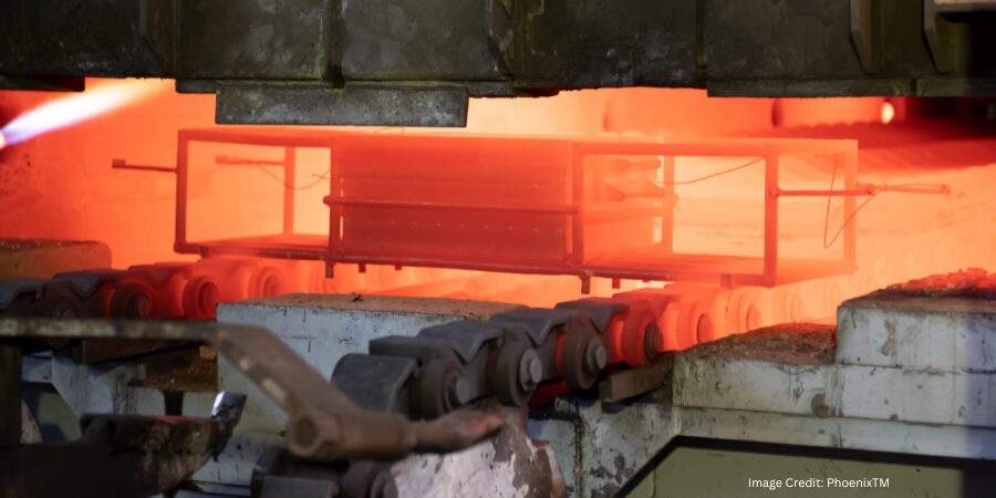
Much of our focus is on heat treatment of metals. We are trying to provide different solutions across the whole gamut of the heat treating industry — from primary production, such as slab heat treatment for steel and for aluminum, proving that the raw material has been processed correctly in the furnace, to the finished product.
We are talking about the formed metal product, making sure that that is achieving the right primary metallurgical properties. It needs to do the function it’s going to be used for, from a temperature profiling perspective and also possibly even a temperature uniformity survey (TUS), which is obviously critical in many of the automotive and aerospace sectors of the market where they’re trying to prove or validate the furnace performance.
What is Thru-Process Monitoring? (6:08)
Heather Falcone: Can you explain what thru-process is and how it influences the monitoring technology that you’re talking about?
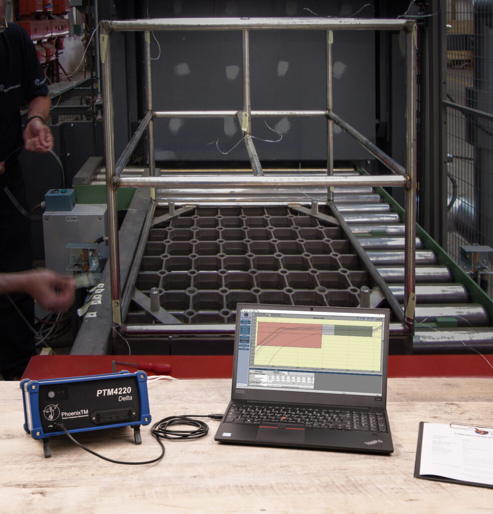
Steve Offley: “Thru-processes” is the term that is key to the type of solution we are trying to provide. When we’re talking about heat treatment, there are still many applications where the product may be heat treated in a static box furnace, in which case the traditional technology of using trained thermocouples is probably as easy as any other, whereby you have your field test instrument external to the furnace chamber. The thermocouples are then moved into — or traced into — the furnace, attached either to the product or, if you’re doing a thermal uniformity survey, to a test frame to locate the thermocouples at the desired coordinates within the working zone of the furnace. Then you are collecting the data externally.
I believe it was two episodes ago that you had Dennis from ECM talking about modular heat treatment. He was talking about the challenges of or the increased level of technology associated with moving batches of products around the heat treating cycle in a modular approach.
When you have that type of setup, and even in situations where you may be heat treating in a continuous furnace, the use of a trailing thermocouple becomes difficult at best, impractical and problematic in terms of safety at worst. For the modular approach, you have thermocouples going into different chambers and moving around. There are seals and automated doors in which the thermocouples will be trapped. As such, it’s very difficult to actually monitor the whole sequence of events that may be occurring in the heat treatment sequence.
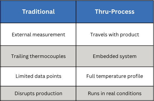
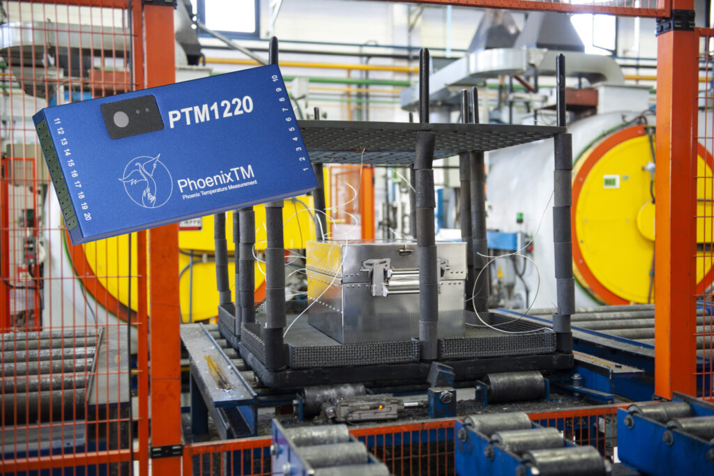
This brings us back to the thru-process methodology. At Phoenix, we offer a system that is designed to travel as if it was part of the product basket through the process. The field test instrument, the data logger, has to travel with the product through the furnace.
A data logger in its own right is not capable of going through a furnace if you are measuring at 800°F to 1000°F. One of the key aspects of our system solution is what we refer to as the thermal barrier. It is an enclosure that is used to protect the data logger to allow it to travel through the process. Essentially you encase the data logger inside the barrier and then place it on the conveyor or in the product basket with short thermocouples that are then rooted to the product or to the test frame that’s being moved with the whole monitoring system through the process.
The Importance of Thermal Barrier Design (9:38)
Heather Falcone: The thermal barrier design is really important then, because you’re going to see a variety of environments. How do you protect the data logger?
Steve Offley: That’s the crux of the technology that we’re trying to provide, in so much that there are many different forms of heat treatment or many different forms of thermal processing where we’re trying to provide the protection we need.
You may have, for instance, a low pressure carburizing process where you’re putting the system into a vacuum furnace, and then you may have a high pressure quench at the end. You have to protect the logger and not just from the temperature criteria inside the furnace, but certain things like pressure changes, which can distort the equipment. That is one design barrier, which would give additional protection to prevent any distortion or compressional damage to the barrier.
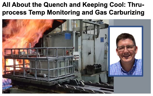
There may be some circumstances, like with a T6 aluminum process, where you have sent the system through the furnace, you then got a water quench, and now in the thru-process principle, the equipment has to go through all aspects of the process. You therefore have to have a design in which the system can tolerate both the heating process, but also the rapid cooling going into the water.
You may also have a situation where you have an Endothermic carburizing furnace with an integrated oil quench. The same approach applies. You are going from a hot environment and then rapid cooling. You are not only protecting the logger from the damage of the heat, but also the materials, like the oil or water in the water sequential and oil quench scenario, so as to not damage the fairly sophisticated electronics of the data log.
There is a lot of science and technology involved in designing unique solutions to meet the specific requirements of the applications. In most cases, we are working with the client from their working spec to develop unique solutions that will meet their unique requirements.
Protection and Accuracy (13:36)
Heather Falcone: When we’re talking about actually monitoring the surveys, what special measures are you required to design the data loggers with that provide accuracy?
Steve Offley: By the very nature that we are sending the data logger through the furnace, we have to be careful that we are not only protecting the data logger from physical damage, which is possible if we do not get the thermal barrier design correct. But we also want, at the end of the day, to guarantee that we are achieving the accurate data that we need to make sense of the profile information that we are getting. Because at the end of the process, you either have the thermal fingerprint of your process or if you’re doing temperature uniformity survey, you have the readability of the data at the respective test levels. According to the standard CQI-9 and AMS2750, the accuracy of the reading or the field test instrument has to be within ±1°F.
The purpose of the barrier is to not only protect the data logger from damage, but keep the data logger at a working temperature that allows the accuracy of the reading that conforms to the standards that you are working to.
There are different designs of thermal barriers that we can offer. The basic design is what we refer to as the microporous insulation technology. This is basically a dry barrier whereby the insulation slows down the penetration of the heat to the core of the barrier where the data logger is. But at the center of that barrier, there will be a device that we refer to as a heat sink. There’s a eutectic salt inside the heat sink, which will transfer its physical state from a solid to a liquid at a nominal temperature. It’s 58°C where the transfer occurs and that will maintain the temperature at that working temperature.
For longer processes, you may want to use a thermal barrier that uses what we call a phased evaporation protection methodology. In simple terms, it involves the use of water, which is able to absorb very large amounts of energy and heat, and obviously will boil at 212°F (100°C). While it’s maintaining that boiling state, it will maintain the temperature of the thermal barrier and the data logger inside it. So we can actually offer a high temperature data logger that is capable of operating safely at 212°F for long periods time and still be protected.
Thermocouple Use (17:00)
Steve Offley: As long as the barrier provides us with that thermal protection and the logger is working within its operating range, we are fairly safe. That being said, we have to be a little bit careful when we consider the technology of the thermocouple, because there’s some fairly serious restrictions on thermocouple use, which many people may or may not be aware of.
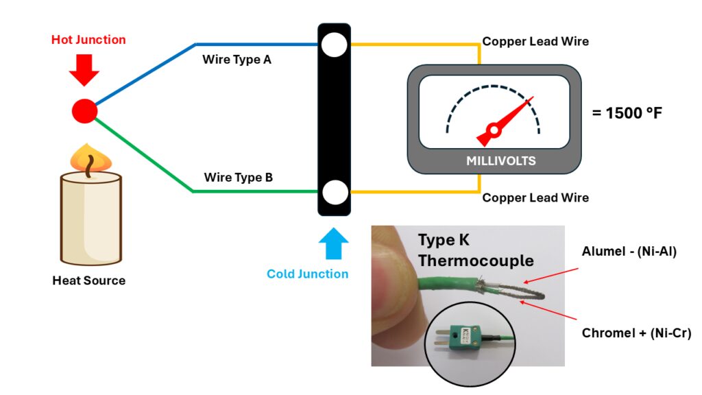
Many people know that the thermocouple technology was developed by Dr. Seebeck back in about 1821. He was a German physicist who discovered the fact that if you had two dissimilar metals connected at a junction or a point, at a particular temperature, those two dissimilar metals would create a millivolt reading, and that millivolt reading would be proportional to the actual temperature that those two dissimilar metals were experiencing. Hence the theory of the thermocouple.
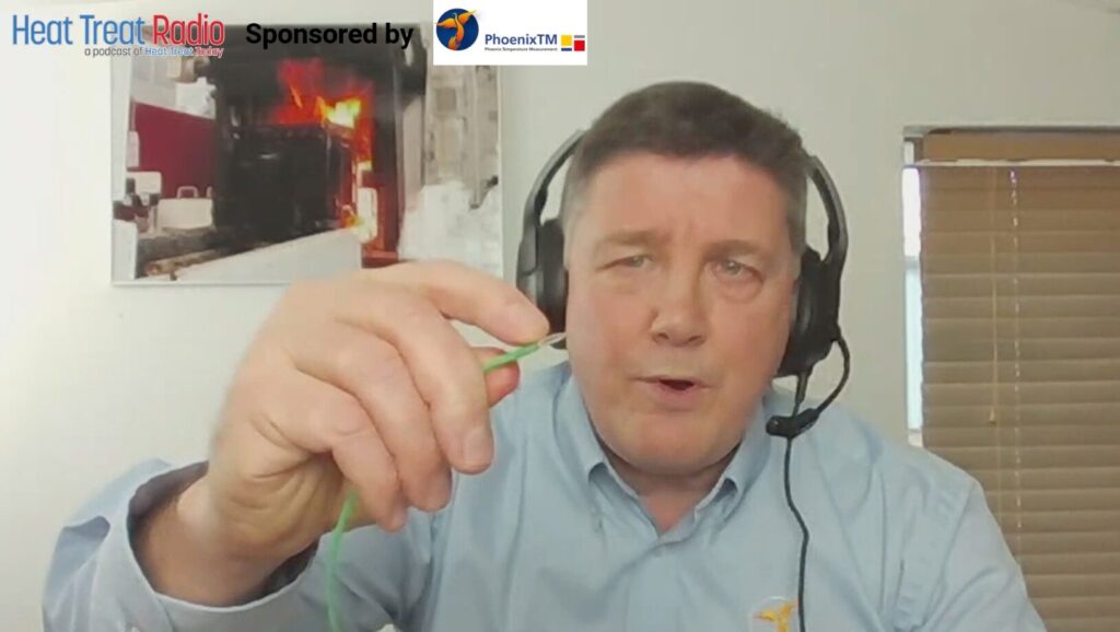
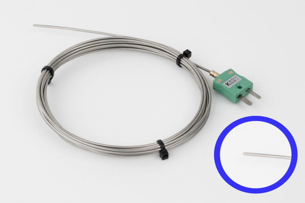
Most people are fully aware of what a thermocouple looks like, but it’s important to note that this is a type of thermocouple we’d use for a coating application. It has a PFA-insulated sleeving on it. You would not use this in many heat treatment applications, but what I want to do is to show you that in the core of the thermocouple, there are two wires, two dissimilar metals. This is a type K thermocouple. We have the aluminal and the chromal leg of the thermocouples. These are the unique materials that are used to generate the millivolt reading.
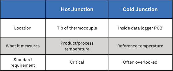
The way the thermocouple works then is that that millivolt can be cross-referenced to a calibration table or a voltage table to determine the temperature reading that the sensor. This is what we refer to as the hot junction, the very tip of the thermocouple. It’s critical that that point is where you want the measurement to be made.
What is often missed is the fact that with a thermocouple, although the hot junction is critical, there is another junction that is even possibly more critical and sometimes overlooked — the cold junction. The thermocouple does not actually record an absolute reading, it’s a ratio between the hot junction and the cold junction. The cold junction of a thermocouple is where the actual thermocouple materials, the two dissimilar metals, join what we refer to as the copper connection. This tends to be where, in the data logger or the field test instrument, the electronics make the physical measurement or process the actual reading from the thermocouple.
If you have a fixed data logger like we have at Phoenix, whereby you would designate the type of thermocouple you were plugging into the data logger — this is a data logger with 20 channels and it’s a type K — I would plug my thermocouple simply into that connector. The cold junction is not in this case at the point where I’m making the connection on the data logger. It is actually inside the logger because there is another wire that goes from the socket to the PCB board where the measurement is actually taken.
Inside the data logger, there is a connector block where the thermocouple wires from the thermocouple sockets will all join the PCB board where the measurement is taken. That’s the location where the cold junction measurement is taken. So, we have our hot junction at the end of the thermocouple, and we have our cold junction inside the data logger.
For some data loggers, that connector or that coal junction may actually be on the outside of the data logger, if it’s a universal connector. So it’s important that you understand where that cold junction is in-situ within your technology. The importance of the reading is the fact that you have a ratio between the hot junction where you are measuring the product and the cold junction where that physical measurement is being referenced inside the data logger.
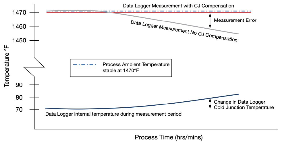
You can imagine, therefore, if the data logger temperature changes, that change in data logger temperature can actually affect the reading you are taking inside your process. That is why it is important to either understand that and make changes so it’s prevented or do what we refer to as cold junction compensation.
Cold Junction Compensation (22:35)
Steve Offley: Inside the data logger, if you are going to compensate for that temperature difference, the data logger is protected up to a physical temperature. But the temperature is going to change. So that cold junction is going to change as it travels through the processing in the way that we do our measurements for thru-process monitoring. The logger will rise in temperature. Therefore, we have to compensate for that.
In the center of the data logger where the connection is made with the copper from the thermocouple cable to the copper-copper connection, we have a temperature sensor, a thermistor, which is accurate to 0.18°F. It measures the actual cold junction temperature of the logger, and it will then compensate automatically for that. Therefore, you can guarantee that even when your data logger temperature changes temperature, it’s compensating for that. There will be no drift in the measurement temperature that you are measuring at the hot junction at the product level.
Heather Falcone: That was the first time that I had read about the cold junction compensation and why it’s so critical, especially when we’re doing TUS activities.
Steve Offley: With TUS, the accuracy of both the data or the field testing instrument, or the data logger and the thermocouple, are critical to the quality of the test data that you are collecting and obviously trying to comply with the very stringent requirements of the AMS and the CQI-9 standards.
In our case, where we are going through the furnace, we have a worst-case scenario because the data logger is naturally going to change in temperature. But even if we take the scenario to the shop floor, and we are doing an external temperature uniformity survey, the data logger that is sitting outside the furnace, cold junction compensation is still critical for that because within a working day, the floor temperature is generally going to be changing.
Events on the shop floor, like opening the furnace activity on the shop floor, are going to change that temperature. I’ve been in many plants where seasonal changes can make a significant difference to the temperature into which you are taking the temperature. It won’t be the first time I’m sure that people have taken equipment out a car after having traveled for many miles in the early hours of the morning only to realize that the data logger temperature may not be at room temperature. You have to be very careful that you have a stable piece of equipment and that the cold junction is working correctly.
It’s important to read the user manual because there’s often a very critical step to make sure that you are either calibrating the equipment in a real-life environment where the temperature change may be, or ensuring sure that your system has got cold junction compensation. Otherwise, what you believe is a true measurement and accurate, may be the calibration laboratory accuracy where the temperature is controlled very, very strictly. In a real life situation, you may not be seeing exactly the same results.
Heather Falcone: It is really important to consider because there are specific accuracy considerations for AMS2750 and CQI-9.
Steve Offley: I often make an analogy to racing. The Formula One racing cars are tuned up to perform highly on a racetrack environment. They can do 200 miles an hour, having been finely tuned, and they work well. If you take that same racing car off the road into the countryside, it is not going to be working quite as effectively.
The same can be said for data logger technology. A data logger that works well in a calibration laboratory and under fairly safe conditions may or may not be working as effectively on the shop floor, particularly when you consider the variation and the challenges that that environment will bring to a measuring system like this.
Linear Interpolation Correction Factor Method (27:22)
Heather Falcone: Can you explain how you use the linear interpolation correction factor method, because that’s one of the only that is allowed by AMS2750, and why it is beneficial to your data quality?
Steve Offley: We discussed the nominal requirements for the data log accuracy for its measurement, but for AMS2750, logger correction factors and also thermocouple correction factors can be applied to the test data that you are collecting with your monitoring system.
Firstly, for the data logger, we can create a data logger correction factor file, which basically shows the correction factors that need to be applied to each of the separate channels of the data logger for the data that you are collecting. Inside the data logger, we store the calibration information that was gleaned in the calibration laboratory. That can then generate an automatic calibration template, which can be automatically applied to each one of the channels on the data logger automatically as part of the test routine.
The last thing we want to do is to make some error by transferring raw data manually from a spreadsheet into a piece of software. So, the nice thing about that is that it’s automatically applying the pre-programmed offsets from the calibration routine in the laboratory itself.
Secondly, with the thermocouple, we can take a calibrated thermocouple where there will be a nominal reading at two ends of the thermocouple, and you then get the average correction factor. In some circumstances, people will apply a thermocouple correction factor of one nominal temperature below the test level that they are applying. At Phoenix, we calibrate the thermocouples across the complete temperature range of the data logger. Then, we apply what we call the linear interpretation method. What that means is that between each calibration point, we can calculate, using a linear regression line, the true correction factor at any temperature over the measurement range of the device itself.
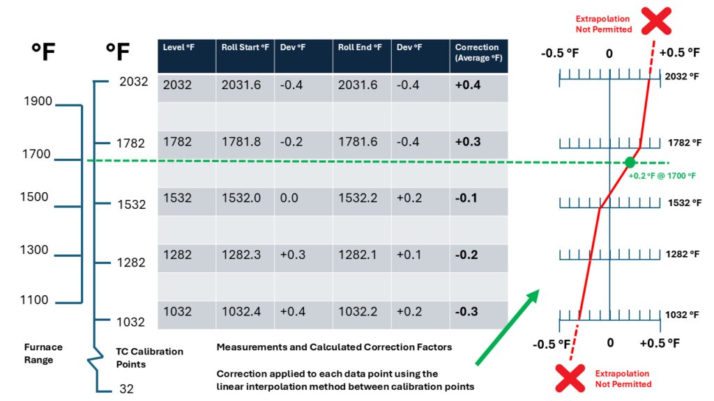
It cannot go beyond the bounds of the upper and lower limit, as extrapolation is not allowed as it says in the standard. But within the upper and lower bounds, we can interpolate linearly between each data point. There is a tight 140° between each point that we can then ensure that we are correcting for or playing the correct correction factor at each temperature from start to finish, not a nominal value over the whole range. In our view, that gives a far more accurate interpretation of the corrected data over the complete working range of the system as opposed to a single nominal value.
Final Thoughts (31:09)
Heather Falcone: We have talked about a variety of topics: thru-processing monitoring, thermal protection at the data logger, the benefits of making sure that you apply cold junction correction, and the specific accuracy considerations that we have to make sure we bundle in all together. What is the big takeaway you want to leave us with?
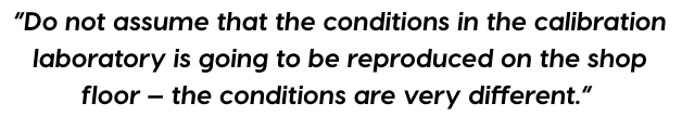
Steve Offley: Be careful you do not assume that the condition of operation in the calibration of laboratory is going to be reproduced on the shop floor because the conditions are very different. This comes back to the argument for the importance of cold junction compensation. If you are using technology or a data logger, check with the manual for what cold junction compensation should be applied and if there are any steps you need to make to ensure that that is applied correctly on the shop floor. If you do not, there is a high risk that what you think is accurate data may or may not be if you have a situation where your data logger temperature is varying with time, either in process or even on the shop floor with changing environmental conditions.
Heather Falcone: In the end, we want to make sure that we’re making good parts, and this sounds like a great system to make sure that you’re getting as accurate as possible.
Steve Offley: Quality data at the end of the day is essential for you to understand what your process is doing. It’s no good relying on data you cannot trust. Take that extra time to investigate and put steps in place to make sure that you are measuring what you think you are measuring at the hot junction and that the cold junction is being considered as part of that measurement process.
About the Guest

Product Marketing Manager
PhoenixTM Ltd.
Dr. Steve Offley, aka “Dr.O” is a product marketing manager with PhoenixTM Ltd. with 30 years of experience of temperature monitoring in the industrial thermal processing market.
For more information: Contact Steve Offley at steve.offley@phoenixtm.com.