
What data can be gleaned for optimizing charge combinations? Check out this Technical Tuesday installment, by Tim Kaufmann and Dierk Hartmann, of Hochschule für angewandte Wissenschaften Kempten; Shikun Chen and Johannes Gottschling, of Universität Duisburg-Essen.
This article showcases the utilization of data-driven modeling assisted by machine learning (ML) to simulate the melting process of different steel grades in a medium-frequency induction furnace concerning the target variable of energy consumption. The results of the predictive models developed are presented in this article, along with the possibility of producing optimized charge combinations through the use of predictive outcomes and backward analysis.
This informative piece was first released in Heat Treat Today’s April 2025 Annual Induction Heating & Melting print edition.
Introduction
The steel and foundry industry faces several ongoing challenges, such as escalating costs of raw materials and energy, CO2 emission regulations, and fierce global competition. To tackle these challenges, there is a continual demand for improving current production processes. Despite the strides made by smelters and equipment manufacturers in enhancing plant technology, there is still room for improvement in production procedures and processes. One possible approach to enhancing these processes is through modeling.
In recent times, digitalization and machine learning (ML) have emerged as a promising modeling method, as demonstrated in material development or process optimization in the steel industry (Lee et al., “A Machine-Learning-Based Alloy,” 11012; Klanke et al., “Advanced Data-Driven Prediction,” 1307-1313; Yingjun et al., “A Machine Learning and Genetic,” 360-375.) The subsequent example showcases how the melting process in a medium-frequency induction furnace can be modeled with respect to energy consumption, using specific process data obtained from a steel foundry, and subsequently optimized through synthetic data generation and backward analysis.
Modeling
Various ML algorithms [including Random Forest, Extra Trees, LightGBM, XGBoost, MLP (Neural Network), K-Nearest Neighbors] were trained and their hyperparameters optimized for modeling Erikson et al., “Autogluon-tabular”. The hyperparameters are set before the learning process begins and influence how well a model can represent a process. Some examples of hyperparameters in ML are the learning rates, the number of hidden layers in a deep learning neural network, or the number of branches in a decision tree.
For the modeling, data from the process, induction furnace, and charge database of a medium-sized steel foundry were consolidated and pre-processed. The melting unit is a medium-frequency induction furnace with a capacity of approximately 7 tons. Figure 1 depicts an overview of the modeling workflow. The process and furnace databases contain data, such as the chemical analysis of the input raw materials, the measured melting time, and the measured melting energy requirement of the respective melts. The required melting energy (kWh), the required melting time (min) to reach the required tapping temperature, and the alloy quantities (Co, FeCr, FeV, FeSi, etc. kg) to be added after the melting process to correct the chemical analysis were selected as target values. The charge database contains data on the charge scrap for each melt, with details of its quantity and chemical analysis.
At the foundry, the scrap is roughly pre-sorted in separate bins so that the scrap used in a batch can be distinguished. As an intermediate step, the expected melting enthalpy of the scrap was calculated from the chemical analyses using simulation software (CALPHAD method). Based on the thermodynamic data, an ML model was trained to also consider the theoretically required melting enthalpy of the raw materials based on the chemical analysis. The measured raw data consist of approximately 10,000 individual melts of different steel grades. After pre-processing (removing outliers, formatting the data, etc.) and applying domain knowledge, about 70% of the data was used for process modeling. Domain knowledge in this context means reviewing and filtering the data with an understanding of the process. For example, some obvious outliers or erroneous data, such as negative charge quantities or charges of allegedly more than 7 tons of material, were not detected by the pre-processing algorithms and were manually filtered out.
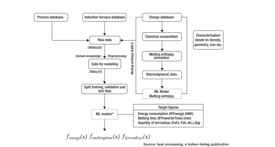
The remaining dataset contains information on approximately 7,000 individual steel melts with approximately 300 influencing variables (columns in the dataset influencing variables, also called “features”) of which approximately 200 are charge-relevant influencing variables. In addition, the steel scrap was divided into groups, such as recycled or foreign scrap and alloys, characterized based on its empirically assessed geometry (cut-offs, “bones,” plates, chipped scrap, etc.), and added to the dataset as information.
The data were subsequently split as 70% training, 20% validation, and 10% test data. The algorithms were trained on the training data and then tested for prediction quality on the test data. This step is necessary because overfitting or underfitting can occur when training ML algorithms. This means that the models perform well on the training data but poorly on unknown future process data. The test data, representing completely unknown future process data or states, are separated beforehand. In each case between the prediction of the model and the “real” measured value of the respective melt in the test dataset, the prediction of the models was evaluated with the metrics MAE (mean absolute error), MSE (mean square error), RMSE (root mean square error), and R2 (coefficient of determination).
The energy consumption during melting in an induction furnace depends on many factors, such as the raw materials being fed (fine or bulky material, impurities, etc.), the sequence in which they are charged, the actual process control (e.g., is the furnace lid open for an unnecessarily long time due to bulky scrap in the charge), and many other direct and indirect influencing factors. Due to this complexity, modeling
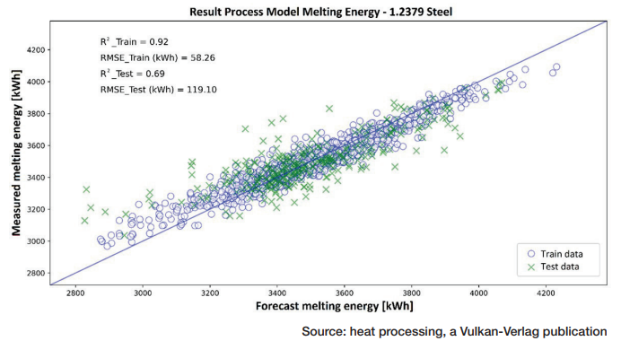

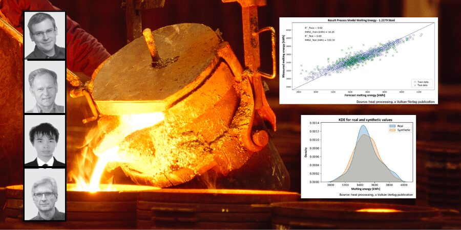
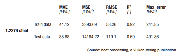
Figure 2 depicts the comparison of the values (1.2379 steel) of energy consumption (x-axis) predicted by the best ML model based on the input features and the actual measured values (y-axis) in the test and training datasets, respectively. For the training dataset the R² is 0.92 with an RMSE of 58 kWh, and for the test dataset, the R2 is 0.69 with an RMSE of 119 kWh (Table 1). For the test data, this corresponds to a relative prediction error of about 5%–10%.
Figure 3 illustrates the residual distribution (difference between the actual measured value and the model prediction) of the 1.2379 energy model in the test dataset. The residual distribution gives an indication of the prediction quality of a model. If the expected value of the residuals is not close to zero and they are not approximately normally distributed, this means that the model has a systematic tendency to either over- or under-predict. Furthermore, if there is a pattern in the residuals, the model does not appear to be able to explain some relationships within the data and is therefore qualitatively inconsistent. In the generated model, the residuals are almost normally distributed, and the prediction error does not appear to follow any pattern, suggesting good prediction quality.
Charge Optimization
After a trained ML model has been prepared for use, backward analysis can be applied to the training dataset to determine the range of values of the independent variable that corresponds to a given target variable. Consequently, backward analysis offers an inverse function of the prediction function, which can be leveraged to determine optimized process values. In this scenario, the optimized process value is the charge composition, with the target variable being energy consumption.
There are multiple mathematical optimization methods that can be employed for this purpose based on a well-trained ML model. A straightforward and easy-to-understand approach is to create a dense set of independent process variables using linear interpolation within a given range, such as the minimum and maximum values of a variable. The target variable is subsequently predicted based on this set of generated variables. This method can be computationally intensive and time consuming, and it does not consider the hidden patterns within the dataset, resulting in some useful information being disregarded.
In order to capture the hidden information and accurately reflect the true value of the original data set, a deep learning-based method called SDV (Synthetic Data Vault) is used in this work Patki et al., “The Synthetic Data Vault,” 1-10. Various synthetic data generation algorithms, such as Gaussian copula, are used in the SDV library. Mathematically, a Gaussian copula is a distribution over the unit cube between 0 and 1 in dimensions generated by applying the probability integral transformation to a multivariate normal distribution over all real numbers (R). Intuitively, the Gaussian copula is a mathematical function that can describe the joint distribution of several random variables by analyzing the dependencies between their marginal distributions. It can learn the intrinsic information of the original dataset to generate new synthetic data that have the same format and statistical properties as the original dataset.

Since the SDV library learns probabilistic rules, most of the synthesized data is general. To improve the quality of the synthesized data, some technical constraints can be defined when generating the data. For example, constraints can be set so that the values of a column in the generated data set are always larger or smaller than another column. Figure 4 shows the comparison of the Kernel Density Estimation (KDE) of the target variable energy consumption in the real and synthetic data. The distributions are very similar. In the current production process, the SDV dataset can be used to quickly determine the values that best approximate the required quality according to the prediction for the independent variables. This selection can then be further optimized, for example, in terms of cost and energy efficiency.
Figure 5 illustrates the process of backward analysis and resulting optimization based on the target, the required chemical elements, and the amount of scrap that must be included in a melt to ensure the target composition. The aim of data-driven optimization is to determine the most cost-effective scrap mix or “recipe,” taking into account the predicted energy consumption and metal yield. The database, which contains information from scrap suppliers, is constantly updated and fed new data. Because of this, the results of the optimization are automatically adjusted on an ongoing basis.
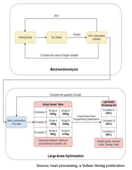
The solution to the programming problem should indicate from which scrap supplier and which type of scrap combinations should be purchased to maintain the desired stock levels of the steel producer that will meet the above conditions (desired chemical analysis, minimized energy consumption, post-gating with ferro-alloys) or minimize costs Goutam and Fourer, “A Survey of Mathematical Programming,” 387-400.
The availability of individual scrap suppliers, the market price, and the levels of elements, such as chromium, vanadium, sulfur, and phosphorus, all affect how economically recovered steel scrap can be used. To ensure that steel grades are consistent throughout the cast or semi-finished product and to meet a client’s criteria, such as weldability and hardness, it is critical to control the amount of these elements in the final melt.
A model-based linear first-order (LP) optimization problem has been developed as a tool for scrap purchasing decision makers Applegate et al., “Practical Large-Scale,” 20243-20257 and Miletic et al., “Model-Based Optimization,” 263-266. The computations are performed by the model using the results of the ML model shown earlier in terms of energy consumption and scrap quality data, market prices, and supplier availability information. Prices, quality, and supplier information are included in the model along with quality and density constraints and a production schedule. The LP considers the following convex quadratic programming problem:
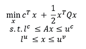
where A is an m × n Matrix and Q is a symmetric and n × n positive semidefinite matrix. The vectors of the input features have the upper bounds uc and uv and the lower bounds lc and lv , which have values in R U+∞ and in R U–∞ respectively. This equation assumes that lc ≤ uc and lv ≤ uv. For example, it can take into account that a particular scrap is only used between 500 kg and 1,500 kg, which may be due to process-related circumstances, and is therefore added as a constraint to the optimization objective.
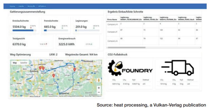
An approximate linear cost equation is used in the model. Scrap costs are determined by market prices and availability, as well as internal storage costs; energy costs are calculated by estimating the energy consumption predicted by the ML model for each type of scrap and the amount of electricity required. The work described above ends with a web-based user interface (Figure 6) that displays the concrete purchase plan. Transportation of the purchased scrap could be considered through route planning. Finally, an estimate of the quantitative carbon footprint of the melting process and the logistics of scrap delivery can be calculated and tracked.
Conclusion
This article has shown how the melting and purchasing process in the steel industry can be modeled and optimized using modern methods from the field of artificial intelligence and mathematical optimization methods. Based on the input features (the scrap composition and the process parameters), the generated models can predict the expected energy consumption with a relative error of about 5%–10%. The optimization software can then be used to generate a scrap composition. Here, the composition of the purchase list from a purely monetary point of view (scrap prices) is supplemented by the consideration of resource and energy efficiency.
The foundry and steel industry naturally must go through a large number of (partial) processes on the way from raw material to finished casting or semi-finished product, where a large amount of production data is generated. For a future data-driven optimization of foundry processes, it is therefore necessary to consolidate this data to make the available knowledge usable for process optimization with the help of tools such as ML. This can provide foundries and their staff with another useful tool, like casting simulation, to further improve existing processes and procedures.
References
Applegate, David, Mateo Díaz, Oliver Hinder, Haihao Lu, Miles Lubin, Brendan O’Donoghue, Warren Schudy. “Practical Large-Scale Linear Programming Using Primal-Dual Hybrid Gradient.” Advances in Neural Information Processing Systems 34 (2021): 20243-20257.
Dutta, Goutam, and Robert Fourer. “A Survey of Mathematical Programming Applications in Integrated Steel Plants.” Manufacturing & Service Operations Management 3, no. 4 (2001): 387-400.
Erickson, Nick, et al. “Autogluon-tabular: Robust and accurate automl for structured data.” arXiv preprint arXiv:2003.06505 (2020).
Klanke, Stefan, Mike Löpke, Norbert Uebber, and Hans-Jürgen Odentha. “Advanced Data-Driven Prediction Models for BOF Endpoint Detection.” Association for Iron & Steel Technology Proceedings (2017), 1307-1313.
Lee, Jin-Woong, Chaewon Park, Byung Do Lee, Joonseo Park, Nam Hoon Goo, and Kee-Sun Sohn. “A Machine-Learning-Based Alloy Design Platform Th at Enables Both Forward and Inverse Predictions for Thermo-Mechanically Controlled Processed (TMCP) Steel Alloys.” Scientific Reports 11, no. 1 (2021): 11012.
Miletic, I., R. Garbaty, S. Waterfall, M. Mathewson. “Model-Based Optimization of Scrap Steel Purchasing.” IFAC Proceedings 40, no. 11 (2007): 263-266.
Patki, Neha, Roy Wedge, and Kalyan Veeramachaneni. “Th e Synthetic Data Vault.” IEEE International Conference on Data Science and Advanced Analytics (DSAA) (2016): 1-10.
Yingjun Ji, Shixin Liu, Mengchu Zhou, Ziyan Zhao, Xiwang Guo, and Liang Qi. “A Machine Learning and Genetic Algorithm-Based Method for Predicting Width Deviation of Hot-Rolled Strip in Steel Production Systems.” Information Sciences 589 (2022): 360-375.
This article content is used with permission by Heat Treat Today’s media partner heat processing, which published this article in February 2023.
About The Authors:

For more information:
Contact Tim Kaufmann at tim.kaufmann@hs-kempten.de
Dierk Hartmann at dierk.hartmann@hs-kempten.de
Shikun Chen at shikun.chen@uni-due.de or
Johannes Gottschling at Johannes.gottschling@uni-due.de